MARL, Part 1: Foundations and Markov Games

The RL foundations note considered one agent improving a policy while the environment stayed fixed. In multi-agent reinforcement learning (MARL), another agent's policy also affects the consequences of an action. We separate this interaction model from the training process, then derive the Bellman equation for a two-player zero-sum game.

Recap: Evaluating a fixed policy

For a stationary policy in the finite discounted MDP of the earlier note,

Here $r^\pi$ and $P^\pi$ average rewards and transitions over that policy's actions. With several agents, fixing all their policies permits the same evaluation; deciding which policies to choose introduces the game-theoretic problem.

Click to enlarge · Scroll sideways on small screens

1. From an MDP to a Markov game

We use a finite, fully observed, simultaneous-move Markov game, also called a stochastic game:

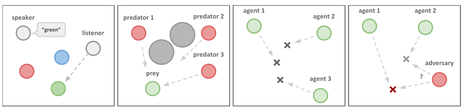
The task sketches above motivate the setting; the proofs below use finite states and actions. Here $\mathcal N=\{1,\ldots,N\}$ indexes agents, $\mathcal S$ is the state set, and $\mathcal A_i$ is agent $i$'s action set. Write $\boldsymbol a=(a_1,\ldots,a_N)\in\mathcal A=\prod_i\mathcal A_i$ for a joint action. The fixed environment satisfies

The public history is $H_t=(S_0,\boldsymbol A_0,\ldots,\boldsymbol A_{t-1},S_t)$. We take rewards to be bounded, $0\le\gamma<1$, and $S_0\sim\rho_0$. All agents observe the current state before choosing their actions; past joint actions are public. They do not observe each other's current sampled actions before choosing their own. Full state observability therefore does not turn simultaneous moves into sequential moves.

This is the model in Hu and Wellman (2003), Definition 2, with the discount and initial law explicit. Littman (1994) connects this framework to reinforcement learning; its main algorithm specializes to two-player zero-sum games.

Scroll horizontally to inspect the full figure →

Policies and the independence convention

A stationary Markov policy is $\pi_i:\mathcal S\to\Delta(\mathcal A_i)$, where $\Delta(E)$ denotes probability distributions on a finite set $E$. A policy profile is $\boldsymbol\pi=(\pi_1,\ldots,\pi_N)$. With independent private randomization conditional on the state,

This product is a modeling assumption, not a consequence of sharing a state. A shared random signal can generate correlated actions: assigning probability $1/2$ to each of $(0,0)$ and $(1,1)$ has uniform individual marginals but is not their product. We use independent policies throughout the equilibrium calculations below.

Write $\mathbb P_{\rho_0}^{\boldsymbol\pi}$ for the trajectory distribution: $S_0\sim\rho_0$, $\boldsymbol A_t\mid S_t\sim\boldsymbol\pi(\cdot\mid S_t)$, and next states and rewards follow the environment's joint conditional distribution. The value calculations use only its state marginal $P$ and conditional reward means $r_i$. These means do not specify the full reward distribution, and we do not assume independent rewards across agents.

Expectations under this profile average over all agents' action draws and environment randomness. The notation $\mathbb E_s^{\boldsymbol\pi}$ fixes $S_0=s$. A superscript containing a deviating strategy replaces the corresponding agent's policy by that strategy.

More generally, a behavior strategy $\sigma_i(\cdot\mid H_t)$ can depend on public history. Stationary policies form a smaller class. We will allow history-dependent unilateral deviations when discussing equilibrium and security guarantees.

2. Evaluating a fixed policy profile

For a stationary profile, define agent-specific values

First, condition the return on the first joint action and next state. The tower property and the Markov assumptions give

Next, define the policy-averaged reward and transition matrix:

Because $P^{\boldsymbol\pi}$ is stochastic and $\gamma<1$, the Bellman-inverse argument applies to each agent:

Once the profile is fixed, all agents share its transition matrix but may have different reward vectors. We can therefore evaluate each return through an ordinary linear Bellman equation. To choose a profile, we must additionally account for agents' responses to one another.

3. Best responses and Nash equilibrium

Let $\boldsymbol\pi_{-i}$ denote every policy except agent $i$'s. Hold these opponents fixed and stationary. Averaging only their actions gives agent $i$ an induced MDP:

Define the best-response value $W_i^{\boldsymbol\pi_{-i}}(s)$ as the supremum over agent $i$'s admissible behavior strategies, with opponents fixed. The finite discounted MDP result gives

The operator on the right is a $\gamma$-contraction: each transition-weighted difference is bounded by $\gamma\|u-v\|_\infty$, and taking a maximum preserves this bound. Its fixed point is unique, and a deterministic stationary maximizer attains it against these fixed opponents. This does not imply that all agents can choose deterministic equilibrium policies simultaneously.

A stationary profile $\boldsymbol\pi^*$ is a statewise Nash equilibrium if

The value on the right is defined by the discounted return under the potentially history-dependent deviation, not by the stationary inverse formula. Equivalently, each agent attains its fixed-opponent best-response value. This is the all-initial-states convention of Hu and Wellman, Definition 3. An equilibrium defined only for $J_i$ at one initial distribution is a weaker requirement.

Reward structure does not determine equilibrium quality

An identical-interest game has $r_1=\cdots=r_N$. A two-player zero-sum game has $r_2=-r_1$. General-sum games impose no such restriction and can contain both compatible and conflicting incentives.

Scroll horizontally to inspect the full figure →

In the coordination matrix, both $(0,0)$ and $(1,1)$ are equilibria: changing one's action alone replaces a positive reward by zero. Yet the former pays each agent $2$ and the latter only $1$. With one self-looping state and $\gamma=0.9$, their values are respectively $20$ and $10$. Nash equilibrium prevents profitable unilateral deviations; it does not maximize a shared return or social welfare.

If a centralized controller can choose every component of a joint action and all agents share a reward, treating $\boldsymbol a$ as one MDP action gives a valid planning reduction. Local information, decentralized execution, and the size of the joint action set are additional constraints, not consequences of reward sharing alone.

4. Why mixed policies can be necessary

Littman's soccer example makes the simultaneous-move distinction concrete. Its state contains both players' positions and ball possession. Each selects north, south, east, west, or stand; the two selected moves are then executed in random order. Collisions can transfer possession.

Click to enlarge · Scroll sideways on small screens

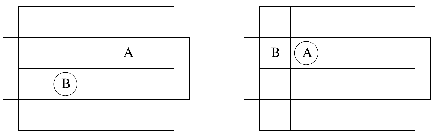
The blocking configuration in Littman, Figure 2 and Section 6.1 motivates randomizing offensive actions. The issue is uncertainty about the opponent's simultaneous move, not an unobserved physical state. We can calculate the same distinction exactly in a smaller game.

Let player 1 maximize the matrix payoff

and player 2 minimize it. If player 1 chooses row $0$ with probability $p$, its expected rewards against pure columns $0$ and $1$ are

A randomized column choice is a convex combination of these two payoffs, so a worst-case column can be chosen pure. Hence

attained at $p=1/2$. Either deterministic row has worst-case payoff $-1$.

Scroll horizontally to inspect the full figure →

With one self-looping state, the uniform stationary policies have value zero for every $\gamma<1$. A deterministic stationary row can be held to $-1/(1-\gamma)$. Randomization here protects against exploitation; it is not merely a temporary exploration device.

5. The zero-sum Bellman equation

Restrict now to two players with $r_1=r$ and $r_2=-r$. At each state, player 1 chooses $x\in\Delta(\mathcal A_1)$ and player 2 chooses $y\in\Delta(\mathcal A_2)$. For a finite payoff matrix $M$, the matrix minimax theorem gives

We use this finite-matrix theorem as a prerequisite rather than proving linear-programming duality here. For a continuation vector $v:\mathcal S\to\mathbb R$, define

The Shapley operator $T$ replaces the single-agent maximum by a mixed matrix-game value. This is the recursion behind Shapley's (1953) Theorem 1 and Littman's Section 4.3.

Shapley's original model uses positive stopping probabilities. A constant stopping probability $1-\gamma$ yields the discounted convention used here; the paper gives this connection in its second example. Our return is the unnormalized discounted sum, not $(1-\gamma)$ times that sum.

A contraction proof

Theorem 1. For the finite discounted zero-sum game above, $T$ is a $\gamma$-contraction in the sup norm. It has a unique fixed point $V^*$, and $v_{k+1}=Tv_k$ satisfies

First, for two matrices $B,C$ of the same size, write $\|B-C\|_{\max}=\max_{a,b}|B_{ab}-C_{ab}|$. Every pair of probability vectors satisfies

For fixed $x$, taking the minimum over $y$ in the inequalities for $x^\top By$ bounds the change in the minimum by the same amount. Taking the maximum over $x$ preserves that bound. Thus

Next, the immediate rewards cancel between continuation matrices:

Combining the matrix-value inequality with this transition bound gives

The finite-dimensional space is complete, so the contraction-mapping theorem gives existence and uniqueness of $V^*$. Repeatedly applying the inequality to $v_k$ and $V^*$ gives the displayed geometric bound. $\square$

Scroll horizontally to inspect the full figure →

Why the fixed point is the game value

Choose optimal matrix strategies $x_s^*,y_s^*$ for $M_{V^*}(s)$. They satisfy the saddle inequalities

Let player 1 use $x^*$ and let player 2 use any history-dependent strategy $\sigma_2$. Conditional on a public history ending in state $s$, the first inequality implies

Multiply by $\gamma^t$, average from $S_0=s$, and sum over $t=0,\ldots,m-1$. The continuation terms telescope:

Since $V^*$ is bounded, the last term vanishes as $m\to\infty$. Reversing the argument with $y^*$ gives, for arbitrary behavior strategies $\sigma_1,\sigma_2$,

Finally, using both stationary strategies gives equality. Thus they form a saddle profile and guarantee the value against history-dependent opponents. This is the stationary-optimal-strategy conclusion of Shapley's Theorem 2, with its discounted telescoping argument made explicit.

6. Planning versus minimax-Q learning

For a known matrix $M$, the maximizing player's matrix-game problem is the linear program

Each inequality protects against one pure opponent action; linearity then protects against every mixed action. The minimizing player has the dual problem. This is the matrix-game computation in Littman, Section 4.1.

Input: Finite two-player zero-sum model $(P,r)$; $0\le\gamma<1$; initial vector $v_0$; iterations $K\ge1$.

Output: Value approximation $v_K$ and residual bound $e_K$.

1. for $k=0,\ldots,K-1$ do
2. for each state $s\in\mathcal S$ do
3. Form $M_k(s)_{ab}\gets r(s,a,b)+\gamma\sum_{s'}P(s'\mid s,a,b)v_k(s')$ for all $(a,b)$.
4. Solve the matrix-game linear program and set $v_{k+1}(s)\gets\operatorname{val}\{M_k(s)\}$.
5. end for
6. end for
7. Perform one further frozen-vector backup to obtain $Tv_K$.
8. Set $e_K\gets\|Tv_K-v_K\|_\infty/(1-\gamma)$.
9. return $v_K,e_K$.

The certificate follows from the triangle inequality and contraction:

Rearranging gives $\|v_K-V^*\|_\infty\le e_K$. This bounds value error when each Bellman update and matrix-game solution is exact. It does not bound how much an opponent could gain against a policy chosen from the approximate values. Approximate matrix-game solutions would also introduce another error term.

Minimax-Q replaces the model expectation by sampled transitions. Given $(s,a,b,R,s')$, its updated entry has the form

This is the construction in Littman, Figure 1. The planning proof above does not by itself prove convergence of this sampled recursion: coverage, learning-rate conditions, and stochastic approximation must also be handled. In a general-sum game, replacing the matrix value by a chosen Nash payoff does not inherit this scalar contraction argument; Hu and Wellman state restrictive additional convergence conditions for Nash Q-learning.

7. Why independent learning can be nonstationary

Concurrent learning can change an agent's expected rewards and transitions even when the physical game remains fixed. These expectations average over the other agents' policies. If those policies are $\boldsymbol\pi_{-i,n}$ at training iteration $n$, then

and $\bar r_{i,n}$ changes by the analogous averaging. One or both can vary with $n$, even though $P$ and $r_i$ do not. This is the distinction behind the nonstationarity discussion in Lowe et al., Sections 1 and 3.

For an exact example, reuse the identical-interest coordination game and let the opponent choose action $0$ with probability $q$. Agent 1's expected immediate rewards are

Therefore action $0$ is a best response when $q\ge1/3$, action $1$ when $q\le1/3$, and both tie at the boundary.

Scroll horizontally to inspect the full figure →

A replay batch generated with $q=0.8$ gives expected immediate targets $(1.6,0.2)$; the current opponent at $q=0.2$ gives $(0.4,0.8)$. The preferred action reverses. Here the state always self-loops, so the example isolates reward drift rather than a changing physical transition law. It invalidates a fixed-target argument for an uncorrected old batch, not every possible replay method.

Conditioning on the full joint action leaves the physical kernel $P(s'\mid s,\boldsymbol a)$ unchanged. A critic target also uses future policies, however, so supplying joint actions does not by itself make that target stationary or establish convergence.

8. Local observations and the next parts

Full observation was an explicit assumption of the proofs above. In a partially observed game, agent $i$ instead sees $O_{i,t}$, generated from the state, and may need a local history

Include locally observed rewards or messages in this history when they contain additional information. A current observation need not be a Markov state, as the partial-observability note explains. The fully observed statewise proofs cannot simply be relabeled with $o_i$ in place of $s$.

Click to enlarge · Scroll sideways on small screens

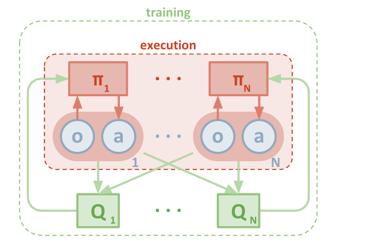
Lowe et al., Figure 1 illustrates centralized training with decentralized execution: critics may use information unavailable to an executing actor. This is a training arrangement, separate from whether rewards are shared, opponents compete, or the agent observes a sufficient state.

Finally, the policy-gradient theorem still provides a useful local connection. With fully observed stationary policies, separate differentiable parameters $\theta_i$, positive action probabilities, and opponents held fixed,

Here $d_{\boldsymbol\pi}=(1-\gamma)\sum_{t\ge0}\gamma^t\mathbb P_{\rho_0}^{\boldsymbol\pi}(S_t=\cdot)$ is normalized. The expectation draws a state from this distribution, then draws each agent's action conditionally on that state. The actions therefore need not be independent of the sampled state.

To obtain the identity, apply the earlier policy-gradient theorem to the MDP with opponents held fixed. Then expand the action value by averaging over their actions. Under the product policy, only agent $i$'s log probability depends on its parameters. The identity gives a partial derivative of that agent's return. It does not prove that simultaneous gradient updates converge to Nash equilibrium.

The remaining parts separate three questions: cooperation and credit assignment; training with information unavailable at execution; and multi-agent actor–critic updates. The definitions here specify which rewards, information, and opponent policies each later method must account for.

References

• Lloyd S. Shapley (1953). Stochastic Games. PNAS, 39(10), 1095–1100. Open paper. Theorems 1–2 and Example 2: value recursion, stationary optimal strategies, and the discount interpretation.
• Michael L. Littman (1994). Markov Games as a Framework for Multi-Agent Reinforcement Learning. ICML, 157–163. Sections 2–5, Figures 1–2, and Section 6.1: minimax policies, linear programming, minimax-Q, and soccer.
• Junling Hu and Michael P. Wellman (2003). Nash Q-Learning for General-Sum Stochastic Games. JMLR, 4, 1039–1069. Definitions 2–3 and the stated qualifications on convergence of general-sum Nash Q-learning.
• Ryan Lowe, Yi Wu, Aviv Tamar, Jean Harb, Pieter Abbeel, and Igor Mordatch (2017). Multi-Agent Actor-Critic for Mixed Cooperative-Competitive Environments. NeurIPS. Sections 3–5 and Figures 1–2: joint-action conditioning, training/execution information, and illustrative tasks. The source's continuous-action methods are not derived in this foundations article.