

Reinforcement Learning: i. Foundations and learning methods · ii. Partial observability, offline data, and DTRs.
An agent may lack access to the environment's full state, or it may have to learn without collecting new interactions. These are different restrictions: partial observability concerns information at decision time, while offline learning concerns access to training data. We derive the corresponding belief-state and off-policy value identities, then connect finite-horizon policy learning to dynamic treatment regimes (DTRs).
Recap: What the fully observed Bellman equation assumes
In Part i, a fixed stationary policy satisfies
Here is an observed sufficient state, its transition kernel, expected immediate reward, and the discount factor. Partial observability changes what information can replace ; offline learning changes how the quantities in this equation can be estimated.
1. Separate the information model from data access
Part i assumed a fully observed Markov decision process (MDP). Its conditional dynamics depended on the current state and action rather than the earlier history. Two separate changes are possible:
| Information available to the policy | New interaction allowed during learning | Fixed logged data only |
|---|---|---|
| Fully observed Markov state | Online RL in an MDP | Offline RL in an MDP |
| Partial observations of a latent Markov state | Online RL in a POMDP | Offline RL in a POMDP |
A partially observable Markov decision process (POMDP) assumes Markov dynamics for a hidden, or latent, state. The current observation need not contain enough information to predict the next observation and reward given the action. Offline datasets can arise from fully or partially observed processes. These distinctions follow Kaelbling et al., Section 3 and Levine et al., Sections 2.1–2.2.
2. Partial observability: Redefine the state and history
Let be a hidden state, an observation, and an action. Rewards are observed. For this section, take all four spaces to be finite and . The finite reward set is a simplifying assumption for the sums, not part of the general definition of a POMDP.
The information available before action is
An admissible policy uses this history, with randomization independent of the hidden state conditional on :
We specify a joint transition–observation–reward kernel
This asserts the latent controlled Markov property and time homogeneity. The initial state has distribution , and is drawn from an initial observation kernel . Together, specifies the model used here.
For a fixed policy, denotes the trajectory distribution generated by , , , and . Probabilities in the belief derivation use this distribution. Conditioning on a realized history averages only over the remaining latent uncertainty and subsequent draws, not over a new history.
The common separate transition/emission notation is a special case. For example, under the corresponding conditional independence assumptions,
The joint kernel retains any information about the hidden state carried by observed rewards. The policy still uses its history rather than assuming that a single summarizes the past.
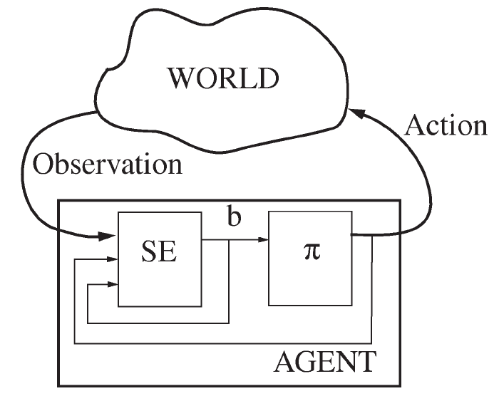
Deriving the belief update
Define the belief state
For an initial observation of positive probability, Bayes' rule gives
First, the policy's information restriction implies that observing the selected action adds no information about beyond :
whenever the conditioning event has positive probability. The law of total probability and the kernel assumption therefore give
Next, define the probability of the next observed pair:
Conditioning on and applying Bayes' rule yields
This update is defined when ; its value at an impossible observation can be assigned arbitrarily. In the transition/emission special case with no additional reward information, this reduces to the usual prediction followed by observation weighting in Kaelbling et al., Section 3.3.
Why the belief is a sufficient state
Write for the updated probability vector. Conditional on , the pair has probability and the next belief equals . Both depend on only through . Thus the belief process is a controlled Markov process.
For example, let be the optimal expected return with decisions remaining, with . Backward induction on this sufficient state gives
Terms with contribute zero. Finally, to prove optimality, consider any history with belief . Its next-outcome distribution is the one derived above, so no randomized action choice can exceed the displayed maximum. Applying the same argument to the remaining decisions proves the claim by induction. A belief-based action attaining the maximum reaches this bound. This is the finite-horizon belief-MDP argument in Kaelbling et al., Section 3.4.
The belief recursion is exact when the specified kernels describe the process. If those kernels are unknown, estimating a belief representation introduces an additional statistical problem.
Example: The same observation can require different actions
Let a fixed hidden state have prior probability for either value. Before a terminal decision, observe three conditionally independent signals, each equal to with probability . There are no informative rewards or choices during this passive observation period. The final action guesses and earns one for a correct guess and zero otherwise.
For a sequence with ones and zeros, conditional independence and Bayes' rule give posterior odds
The histories and have the same current observation , but
The terminal action values are and . The optimal actions are therefore 1 and 0, respectively. A policy using only cannot implement both decisions. A policy using the posterior belief can.
3. Offline is a data-access restriction
For the next derivation, return to a fully observed finite MDP. Use a finite horizon and bounded rewards, so the discount may now satisfy . Policies may depend on the history and decision time. This is a new finite-horizon setup, not an application of Part i's infinite-horizon theorem with .
Suppose a behavior policy generated independent trajectories. The logged dataset is
Rewards and states within a trajectory need not be independent. Offline RL learns a policy using this fixed dataset without further environment interaction for training. Off-policy learning instead describes the relationship between the policy generating data and the target policy; it does not prohibit collecting more data. Levine et al., Figure 1 and Section 2.2 illustrate the distinction.
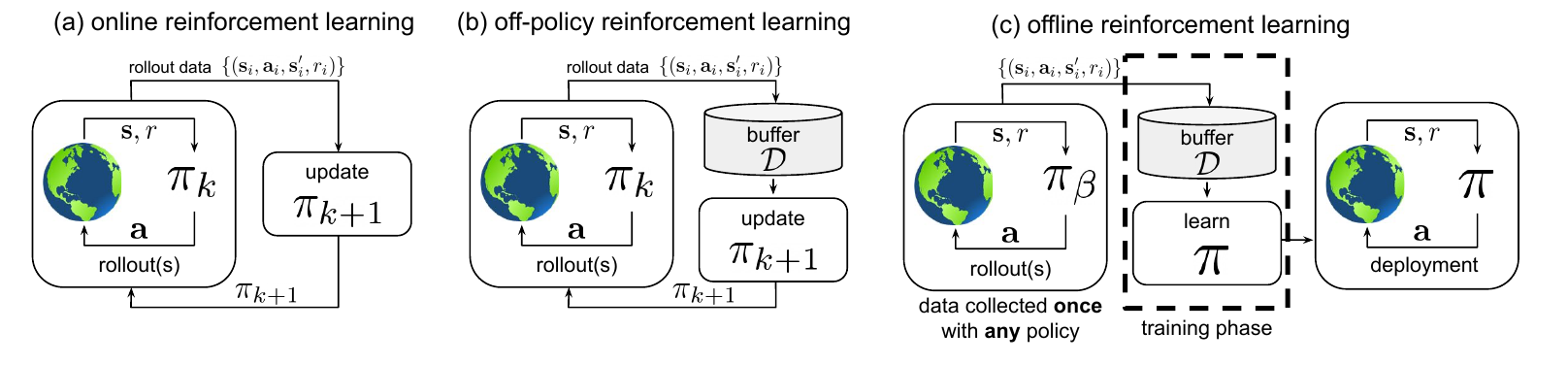
The behavior policy determines which trajectories enter the dataset, whether or not the learning algorithm estimates that policy. We make its role explicit in the value identity next.
An off-policy value identity
For a compact derivation, additionally take a finite reward set and write as a probability mass function. Let and be trajectory probabilities under behavior and target policies, with the same initial distribution and environment kernel:
Let be the trajectory distributions with these mass functions. The dataset satisfies , while policy value averages . Write and , with policies and environment fixed. Neither expectation averages over the process of fitting a policy.
Assume target-policy coverage: implies . In particular, every target action on a target-reachable history must have positive behavior probability. Cancellation of the common environment factors gives
Let . First substitute the ratio, then sum over trajectories:
The second equality uses coverage. This is an identity for a fixed target policy and true trajectory probabilities, consistent with the importance-sampling treatment in Levine et al., Section 3.1. If behavior probabilities are fitted, or the same data select the target policy, additional estimation and data-dependence arguments are required.
Missing coverage is an identification problem
Consider one state, one decision, and two actions. The behavior policy always chooses action 0 and obtains reward zero. Two environments agree on every possible logged observation:
| Environment | Reward for action 0 | Reward for action 1 | Optimal action |
|---|---|---|---|
| 0 | 1 | 1 | |
| 0 | 0 |
The logged-data distributions are identical, but the optimal actions differ. Without additional structural information, no amount of data from this behavior policy can distinguish the environments. A policy choosing action 1 lacks an identified value from these logs.
Even with positive coverage, probabilities can be small. For a fixed time , let and denote the target and behavior state–action distributions. If
then, for any real function on state–action pairs,
This follows by multiplying the pointwise probability inequality by and summing. Large can amplify errors measured under the logged distribution. The inequality explains one role of coverage; it is not by itself a finite-sample policy-learning guarantee.
4. Partial observability is not the same as hidden confounding
The belief update in Section 2 used
This is justified when the agent selects actions from recorded information and independent randomization. It can fail for historical data when the behavior policy uses additional information unavailable in .
For example, if a decision maker observes the hidden state and chooses , then conditioning on the action reveals that state. A posterior that ignores this selection is incorrect. Likewise, the recorded conditional distribution of the next outcome given need not equal its distribution when the action is externally assigned.
To identify intervention values from partially observed logs, we must therefore specify what information the behavior decision maker used. A recurrent representation of or an estimated belief can summarize recorded information, but cannot by itself justify the assumptions needed for causal identification.
5. Dynamic treatment regimes: A finite-horizon connection
Now use treatment stages . Let be information observed before treatment , and let be a bounded terminal outcome, with larger values preferable. For explicit formulas, assume finite covariate and treatment spaces and fully observed trajectories from independent individuals. Define
Each maps the available history to a feasible treatment. This is the setup of Schulte et al., Sections 2–3 and our earlier Q-learning note.
What replaces the latest-state Markov assumption?
A history-based DTR does not require
The transition may depend on all recorded past treatments and covariates. We can still use finite-horizon dynamic programming by taking the whole history, including the stage, as the state. This does not assume that the latest covariate summarizes the past. The history space grows with , so this construction does not provide a low-dimensional state representation.
A terminal-outcome DTR corresponds to the following finite-horizon RL reward convention:
Here RL's action at time is treatment , and its state before that action is . Intermediate utilities can instead be included as rewards when that is the chosen scientific objective.
Causal identification requires separate assumptions
Let denote the outcome under regime , and define its causal value by . Let collect the potential covariates and outcomes under all fixed treatment sequences.
In this section, denotes the logged longitudinal distribution. Unmarked conditional means and treatment probabilities use . By contrast, averages the regime's potential outcome over the baseline population. Equivalently, it averages the terminal outcome under the intervention distribution .
The assumptions below identify from the baseline distribution and the observed conditional covariate and outcome distributions. The treatment rules replace the logged treatment assignments. For the standard no-interference setting, assume:
- Consistency: recorded covariates and outcome equal their potential counterparts under the treatments actually received.
- No interference: one individual's treatments do not affect another individual's potential covariates or outcome; treatment versions are well specified.
- Sequential exchangeability: at every stage. This is a strong sufficient no-unmeasured-confounding assumption.
- Positivity: for treatments required by the target regime on its reachable histories.
These are the identification conditions in Schulte et al., Sections 2–3, not consequences of labeling histories as states. Evaluating one regime requires support for its own treatment choices. Optimizing over all feasible regimes requires support for every candidate treatment on each reachable history.
In the present finite-support setting, positivity gives a positive minimum over the required probabilities. It does not specify how small that minimum may be. Bounds across a sequence of data-generating models often impose a common lower bound . With infinite history spaces, pointwise positivity need not imply such a uniform bound even for a single model.
Under these assumptions, externally assigning the treatments preserves the observed conditional covariate/outcome kernels. For two stages, write
The g-formula is
Consistency links observed and potential variables, exchangeability identifies the intervention kernels, and positivity ensures the required conditionals are supported by the observed distribution.
The DTR recursion is a finite-horizon Bellman recursion
For the unrestricted class of history-based regimes, define
The maximizing rules are , using a fixed action ordering. First, the final rule maximizes the identified conditional terminal mean. Next, its optimized continuation value becomes the outcome averaged at the preceding stage. Repeating this argument backward proves optimality by the tower property and the fact that a maximum dominates any competing treatment choice. The earlier article gives the complete two-stage optimality and estimation-error proofs.
The correspondence is therefore precise: learning a finite-horizon DTR from existing longitudinal data is a history-based offline policy-learning problem, with an explicitly causal value target and identification assumptions. DTRs can also be studied in adaptive or prospectively randomized settings; the entire field is not defined by offline data access.
6. Which distinction determines the method?
| Setting or choice | What must be specified | What does not follow automatically |
|---|---|---|
| Fully observed MDP | Sufficient observed state and controlled transition/reward law | That the model is known or one-step samples are independent |
| POMDP | Latent dynamics, observation/reward information, admissible policy history | That the current observation is Markov or the latent model is identified from logs |
| Offline learning | Fixed data source, target policy class, coverage and estimation conditions | That Markov assumptions disappear or ordinary off-policy updates will suffice |
| History-based DTR learning | Finite-stage decisions, causal outcome, feasible rules, identification conditions | That latest covariates alone are Markov or hidden confounding is absent |
These choices can coexist. A model-based algorithm can learn offline; an actor–critic algorithm can use beliefs; and a DTR can be learned by Q-learning or by the direct-learning methods discussed earlier. The information model, data-access restriction, causal assumptions, and optimization method answer different questions.
References
- Leslie Pack Kaelbling, Michael L. Littman, and Anthony R. Cassandra (1998). Planning and acting in partially observable stochastic domains. Artificial Intelligence, 101, 99–134. Sections 3.2–3.4 and Figure 2 motivate the belief-state construction and controller diagram.
- Sergey Levine, Aviral Kumar, George Tucker, and Justin Fu (2020). Offline Reinforcement Learning: Tutorial, Review, and Perspectives on Open Problems. Figure 1, Sections 2.1–2.4, and Section 3.1 motivate the data-access distinctions, coverage discussion, and importance weighting.
- Phillip J. Schulte, Anastasios A. Tsiatis, Eric B. Laber, and Marie Davidian (2014). Q- and A-Learning Methods for Estimating Optimal Dynamic Treatment Regimes. Open manuscript. Sections 2–3 supply the histories, causal conditions, and backward recursion used for the DTR connection.