MARL, Part 2: Cooperation and Credit Assignment

August 4, 2026

On this page

Part 1 allowed agents to have different rewards. Here they share one reward, but sharing it does not show how each action contributed. We ask two questions: how can an actor compare its action with alternatives, and when can separate agent decisions maximize a learned team value? COMA compares an action with its alternatives while holding teammates' actions fixed. VDN and QMIX instead build a team value from agent-specific scores.

Recap: Why a policy-score baseline can cancel

For a fixed state and a positive differentiable policy, the score identity is

\sum_a\pi_\theta(a\mid s)\nabla_\theta\log\pi_\theta(a\mid s) =\nabla_\theta\sum_a\pi_\theta(a\mid s)=0.

It permits subtracting a baseline that is fixed while this action is averaged. In a team, we must check whether that cancellation remains valid when the baseline also depends on teammates' actions.

1. One reward, several decisions

Consider a finite, fully observed, simultaneous-move cooperative Markov game. There are $N$ agents, state $s\in\mathcal S$ , joint action $\boldsymbol a\in\prod_i\mathcal A_i$ , and one bounded realized reward $R_{t+1}$ received by every agent. The environment is fixed, with joint next-state/reward kernel

(S_{t+1},R_{t+1})\mid H_t,\boldsymbol A_t \sim K(\cdot\mid S_t,\boldsymbol A_t).

Here $H_t$ contains the observed history through $S_t$ ; write $P(s'\mid s,\boldsymbol a)$ for the state marginal and $r(s,\boldsymbol a)=\mathbb E_{(S',R)\sim K(\cdot\mid s,\boldsymbol a)}[R]$ . Take $0\le\gamma<1$ and a fixed initial law $\rho_0$ . Agents use separate parameter vectors $\theta_i$ and positive, continuously differentiable stationary policies, with independent private randomization conditional on the state:

\boldsymbol\pi_\theta(\boldsymbol a\mid s) =\prod_{i=1}^N\pi_{i,\theta_i}(a_i\mid s).

The trajectory law $P_\theta$ is generated by

S_0\sim\rho_0,\qquad \boldsymbol A_t\mid S_t\sim\boldsymbol\pi_\theta(\cdot\mid S_t),\qquad (S_{t+1},R_{t+1})\mid S_t,\boldsymbol A_t\sim K(\cdot\mid S_t,\boldsymbol A_t).

All policy expectations below average over this action and environment randomness, keeping $K,\rho_0$ fixed. Write $P_\theta^s$ for the same trajectory construction with $S_0=s$ fixed, including states outside the support of $\rho_0$ . Suppress the parameter subscript on individual policies when unambiguous. Define

\begin{aligned} J(\theta)&=\mathbb E_{\tau\sim P_\theta} \left[\sum_{t\ge0}\gamma^tR_{t+1}\right],\\ V^\theta(s)&=\mathbb E_{\tau\sim P_\theta^s} \left[\sum_{t\ge0}\gamma^tR_{t+1}\right],\\ Q^\theta(s,\boldsymbol a) &=r(s,\boldsymbol a)+\gamma\sum_{s'}P(s'\mid s,\boldsymbol a)V^\theta(s'). \end{aligned}

Every agent maximizes $J$ , but the shared reward alone does not distinguish the contribution of each current action. Agents may also settle at a suboptimal coordination equilibrium, as Part 1's common-reward matrix showed.

Original Sunehag et al. Figure 3 contains three Fetch and Switch maps and a Checkers map. Gray obstacles create corridors. Colored agents and goals require coordinated movement; green apples and orange lemons in Checkers create different roles for teammates. — **Figure 1. Cooperative tasks in the original VDN paper.** Original figure from Sunehag et al. (2017), Value-Decomposition Networks For Cooperative Multi-Agent Learning, Figure 3. These are the source's task maps, not new simulations. Local observation windows are outlined in the lower-left panel; the note's initial proofs use full-state policies instead. Full resolution ↗Figure excerpt for discussion; copyright remains with the authors/rightsholder.

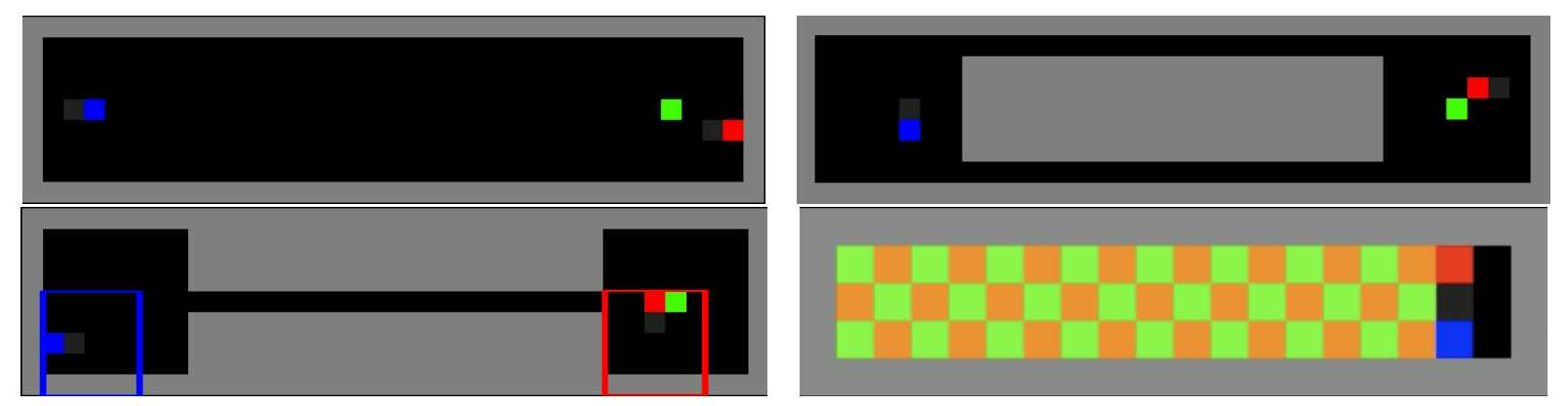
The original VDN tasks illustrate the issue: agents may need to yield in a corridor, coordinate collection and delivery, or clear a path for a teammate. Their reward can depend on actions that work only in combination. The source uses local observations, while our proofs first assume full states. We do not assume that a local observation contains all the information needed to predict the next state and reward.

2. Difference rewards: what changes when one action changes?

At a fixed state $s$ , choose a reference action $c_i$ and hold the other agents' actions $\boldsymbol a_{-i}$ fixed. An immediate difference reward is

D_i(s,\boldsymbol a) =r(s,\boldsymbol a)-r\bigl(s,(c_i,\boldsymbol a_{-i})\bigr).

For two possible actions $a_i,a_i'$ , direct subtraction gives

\begin{aligned} &D_i\bigl(s,(a_i,\boldsymbol a_{-i})\bigr) -D_i\bigl(s,(a_i',\boldsymbol a_{-i})\bigr)\\ &\qquad=r\bigl(s,(a_i,\boldsymbol a_{-i})\bigr) -r\bigl(s,(a_i',\boldsymbol a_{-i})\bigr). \end{aligned}

Thus the reference preserves immediate action rankings at that fixed context. Computing it may require a reward model or a simulator. Foerster et al., Section 4 use difference rewards to motivate a counterfactual critic baseline.

This identity does not justify replacing every reward in a sequential problem by its current-action difference. For example, let $S_0=0$ , $A_0\in\{0,1\}$ , $R_1=0$ , and $S_1=A_0$ . At the final decision there is only a no-op, and $R_2=S_1$ . Then

J(A_0=a)=\gamma a.

Both immediate difference rewards are zero: the first reward is always zero, while the second is independent of the current no-op. Replacing the rewards this way would therefore erase the earlier action's delayed benefit. COMA instead keeps the environment's reward sequence and subtracts a baseline inside its policy-gradient estimator.

3. Counterfactual multi-agent policy gradients

From the team objective to an agent's gradient

Define the normalized discounted occupancy and its joint state-action law:

\begin{aligned} d_\theta(s)&=(1-\gamma)\sum_{t\ge0}\gamma^t \mathbb P_{\tau\sim P_\theta}(S_t=s),\\ \nu_\theta(s,\boldsymbol a)&=d_\theta(s)\boldsymbol\pi_\theta(\boldsymbol a\mid s),\\ \psi_i(s,a_i)&=\nabla_{\theta_i}\log\pi_i(a_i\mid s). \end{aligned}

Sampling $(S,\boldsymbol A)\sim\nu_\theta$ means $S\sim d_\theta$ , followed by $\boldsymbol A\mid S\sim\boldsymbol\pi_\theta$ . It does not mean independent sampling from marginal state and action distributions.

To obtain the gradient, differentiate $V^\theta(s)=\sum_{\boldsymbol a}\boldsymbol\pi_\theta(\boldsymbol a\mid s)Q^\theta(s,\boldsymbol a)$ . Only the policy and continuation value depend on $\theta_i$ :

\begin{aligned} g_i(s):=\nabla_{\theta_i}V^\theta(s) &=h_i(s)+\gamma\sum_{s'}P^\theta(s,s')g_i(s'),\\ h_i(s)&=\sum_{\boldsymbol a}\boldsymbol\pi_\theta(\boldsymbol a\mid s) \psi_i(s,a_i)Q^\theta(s,\boldsymbol a),\\ P^\theta(s,s')&=\sum_{\boldsymbol a}\boldsymbol\pi_\theta(\boldsymbol a\mid s)P(s'\mid s,\boldsymbol a). \end{aligned}

The product policy gives $\nabla_{\theta_i}\boldsymbol\pi_\theta=\boldsymbol\pi_\theta\psi_i$ . Next, use the convergent Bellman inverse, as in the policy-gradient note:

\begin{aligned} g_i&=(I-\gamma P^\theta)^{-1}h_i =\sum_{t\ge0}\gamma^t(P^\theta)^th_i,\\ \nabla_{\theta_i}J &=\sum_{t\ge0}\gamma^t\rho_0^\top(P^\theta)^th_i\\ &=\frac{1}{1-\gamma}\sum_s d_\theta(s)h_i(s). \end{aligned}

Therefore

\boxed{ \nabla_{\theta_i}J =\frac{1}{1-\gamma} \mathbb E_{(S,\boldsymbol A)\sim\nu_\theta} [\psi_i(S,A_i)Q^\theta(S,\boldsymbol A)]. }

Finite states/actions, bounded rewards, and a fixed parameter point with positive differentiable policies justify these derivatives. This is a partial derivative with other agents' parameters fixed, not a convergence claim for concurrent updates.

Why an own-action-independent baseline cancels

Let $b_i(s,\boldsymbol a_{-i})$ be any finite baseline. Under the product policy,

A_i\mid S=s,\boldsymbol A_{-i}=\boldsymbol a_{-i} \sim\pi_i(\cdot\mid s).

First, sum the conditional score over this distribution:

\begin{aligned} \mathbb E_{A_i\sim\pi_i(\cdot\mid s)}[\psi_i(s,A_i)] &=\sum_{a_i}\pi_i(a_i\mid s)\nabla_{\theta_i}\log\pi_i(a_i\mid s)\\ &=\sum_{a_i}\nabla_{\theta_i}\pi_i(a_i\mid s)\\ &=\nabla_{\theta_i}\underbrace{\sum_{a_i}\pi_i(a_i\mid s)}_{1}=0. \end{aligned}

Next, conditional on $(S,\boldsymbol A_{-i})$ , the baseline is fixed. The tower property yields

\mathbb E_{\nu_\theta}[\psi_i b_i] =\mathbb E_{S\sim d_\theta,\,\boldsymbol A_{-i}\sim\boldsymbol\pi_{-i}(\cdot\mid S)} \left[b_i(S,\boldsymbol A_{-i}) \underbrace{\mathbb E_{A_i\sim\pi_i(\cdot\mid S)}[\psi_i(S,A_i)]}_{0}\right]=0.

Here $\boldsymbol\pi_{-i}(\boldsymbol a_{-i}\mid s)=\prod_{j\ne i}\pi_j(a_j\mid s)$ , and $\mathbb E_{\nu_\theta}$ abbreviates the joint expectation already defined. Consequently $Q^\theta$ may be replaced by $Q^\theta-b_i$ without changing the expected gradient. The conditional product assumption is essential to this cancellation with a baseline that depends on teammates' actions.

COMA's choice of baseline

Counterfactual Multi-Agent Policy Gradients (COMA) chooses

\begin{aligned} b_i^{\mathrm{CF}}(s,\boldsymbol a_{-i}) &=\sum_{u\in\mathcal A_i}\pi_i(u\mid s) Q^\theta\bigl(s,(u,\boldsymbol a_{-i})\bigr),\\ A_i^{\mathrm{CF}}(s,\boldsymbol a) &=Q^\theta(s,\boldsymbol a)-b_i^{\mathrm{CF}}(s,\boldsymbol a_{-i}). \end{aligned}

The index on $A_i^{\mathrm{CF}}$ denotes an advantage, not the random action $A_i$ . At fixed $s,\boldsymbol a_{-i}$ , this advantage has conditional mean zero. It compares the sampled action against agent $i$ 's policy-weighted alternatives, holding teammates' current actions and the future policy fixed.

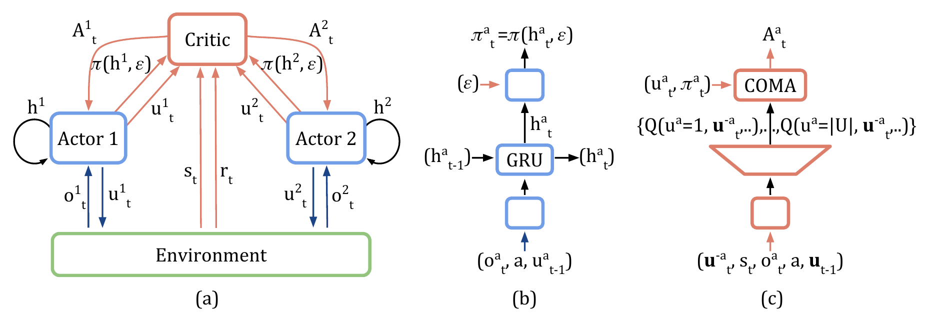
Original Foerster et al. Figure 1 has three panels: two decentralized actors interacting with an environment and a centralized critic; a recurrent actor network; and a critic producing a vector of values for all actions of one agent while holding other agents' actions fixed, followed by the COMA advantage calculation. — **Figure 2. COMA's actors and counterfactual critic.** Original figure from Foerster et al. (2018), Counterfactual Multi-Agent Policy Gradients, Figure 1. The source uses u for actions and local-history actors. Red components are used in centralized training; the derivation in this note specializes to fully observed state-based policies. Full resolution ↗Figure excerpt for discussion; copyright remains with the authors/rightsholder.

In the original figure, panel (c) evaluates all own-action alternatives in one critic pass; the paper writes actions as $u$ and uses local histories in the actors. The calculation above is its fully observed specialization. This is a critic-based counterfactual, not a uniquely defined allocation of team reward, a Shapley value, or identification of causal effects from observational data. See Foerster et al., Equation (4).

What an approximate critic does not preserve

For a fitted critic $\widehat Q$ , define $\widehat b_i^{\mathrm{CF}}$ by the same conditional sum. At a fixed policy and fixed critic, its baseline still cancels exactly. However,

\begin{aligned} \widehat g_i&=\frac{1}{1-\gamma} \mathbb E_{\nu_\theta}[\psi_i(\widehat Q-\widehat b_i^{\mathrm{CF}})],\\ \widehat g_i-\nabla_{\theta_i}J &=\frac{1}{1-\gamma}\mathbb E_{\nu_\theta}[\psi_i(\widehat Q-Q^\theta)],\\ \left\|\widehat g_i-\nabla_{\theta_i}J\right\| &\le\frac{ \{\mathbb E_{\nu_\theta}\|\psi_i\|^2\}^{1/2} \{\mathbb E_{\nu_\theta}(\widehat Q-Q^\theta)^2\}^{1/2} }{1-\gamma}. \end{aligned}

The Cauchy–Schwarz bound shows which error remains after the baseline cancels: the critic's error in predicting action values. If the critic was fitted on data, these expectations condition on it and use a fresh on-policy draw; reusing dependent training samples needs a separate argument. During the actor update, we treat the critic and baseline as fixed multipliers, even if their values depend on $\theta$ .

4. A worked variance calculation

Consider a one-decision team with independent $A_1\sim\operatorname{Bernoulli}(p)$ and $A_2\sim\operatorname{Bernoulli}(q)$ , where

R=A_1+4A_2,\qquad p=\tfrac14,\quad q=\tfrac12.

For agent 1, take $p=\operatorname{sigmoid}(\theta_1)$ , so its scalar score is $\psi_1=A_1-p$ . Since $J=p+4q$ ,

\frac{\partial J}{\partial\theta_1}=p(1-p)=\frac{3}{16}.

The COMA baseline is $b_1^{\mathrm{CF}}(A_2)=p+4A_2$ . Thus

\begin{aligned} R-b_1^{\mathrm{CF}}&=A_1-p,\\ Z_{\mathrm{CF}}:=\psi_1(R-b_1^{\mathrm{CF}})&=(A_1-p)^2,\\ \mathbb E[Z_{\mathrm{CF}}]&=p(1-p),\\ \operatorname{Var}(Z_{\mathrm{CF}}) &=p(1-p)^4+(1-p)p^4-p^2(1-p)^2\\ &=p(1-p)(1-2p)^2=\frac{3}{64}. \end{aligned}

All expectations and variances in this section use the stated joint Bernoulli law at fixed $p,q$ . Enumerating its four outcomes gives:

Baseline $b$ in $Z=\psi_1(R-b)$	$\mathbb E[Z]$	$\operatorname{Var}(Z)$
$0$	$3/16$	$555/256$
$V=\mathbb E[R]=9/4$	$3/16$	$51/64$
$b_1^{\mathrm{CF}}=1/4+4A_2$	$3/16$	$3/64$
$b_1^*=3/4+4A_2$	$3/16$	$0$

COMA removes variation due to $A_2$ in this example. The final row also shows that its baseline need not minimize variance.

The variance-minimizing conditional baseline

Fix $s,\boldsymbol a_{-i}$ and let only $A_i\sim\pi_i(\cdot\mid s)$ vary. Write $\psi=\psi_i(s,A_i)$ and $Q=Q^\theta(s,(A_i,\boldsymbol a_{-i}))$ . Because $\mathbb E[\psi(Q-b)]$ is independent of $b$ , minimizing the trace of its covariance is equivalent to minimizing

F(b)=\mathbb E_{A_i\sim\pi_i(\cdot\mid s)}[\|\psi\|^2(Q-b)^2].

Differentiate this finite quadratic:

F'(b)=2b\mathbb E[\|\psi\|^2]-2\mathbb E[\|\psi\|^2Q], \qquad \boxed{b_i^*=\frac{\mathbb E[\|\psi\|^2Q]}{\mathbb E[\|\psi\|^2]}}.

This formula assumes a positive denominator. If it is zero, the score contribution is identically zero. COMA uses $\mathbb E[Q]$ instead, so the two baselines need not agree.

COMA also need not reduce variance relative to a zero baseline. With one Bernoulli action and $R=A_1-(1-p)$ , the unadjusted score contribution is the constant $p(1-p)$ . COMA instead gives $(A_1-p)^2$ , which has positive variance when $p\ne1/2$ .

5. Counterfactual actor updates

The following is the actor-gradient calculation, not the complete COMA critic-training procedure. Assume episodic trajectories reach a genuine terminal state with finite expected length, followed by an absorbing zero-reward state. No arbitrary rollout cutoff is inserted.

Algorithm 1 On-policy counterfactual actor-gradient estimate

Input: Frozen policy $\boldsymbol\pi_\theta$ ; frozen critic $\widehat Q$ ; $n$ independent episodes $\tau_k\sim P_\theta$ ; discount $\gamma$ .

Output: Gradient estimates $\widehat g_i$ , one for each agent.

Initialize $\widehat g_i\gets0$ for every agent $i$ .
for $k=1,\ldots,n$ do
for $t=0,\ldots,T_k-1$ do
for each agent $i$ do
Evaluate $q_u\gets\widehat Q(S_{kt},(u,\boldsymbol A_{-i,kt}))$ for every $u\in\mathcal A_i$ .
Set $b_i\gets\sum_u\pi_i(u\mid S_{kt})q_u$ and $\widehat A_i\gets q_{A_{i,kt}}-b_i$ .
Accumulate $\widehat g_i\gets\widehat g_i+n^{-1}\gamma^t\nabla_{\theta_i}\log\pi_i(A_{i,kt}\mid S_{kt})\widehat A_i$ , holding $q_u,b_i$ fixed.
end for
end for
end for
return $\{\widehat g_i\}_{i=1}^N$ .

With $\widehat Q=Q^\theta$ , the episode-average expectation is

\mathbb E_{(\tau_1,\ldots,\tau_n)\sim P_\theta^{\otimes n}}[\widehat g_i] =\sum_{t\ge0}\gamma^t\mathbb E_{\tau\sim P_\theta} [\psi_i(S_t,A_{i,t})A_i^{\mathrm{CF}}(S_t,\boldsymbol A_t)] =\nabla_{\theta_i}J.

The time sum already contains discounting, so no extra $1/(1-\gamma)$ factor is needed. A fitted critic instead has the error described above. Off-policy episodes would require a separate distribution-correction argument. Critic fitting, training/execution information, and concurrent-update stability belong to the later MARL parts.

6. VDN: learning an additive team value

An alternative is to learn action values whose maximization separates across agents. Value-Decomposition Networks (VDN) use

Q_{\mathrm{tot},w}(s,\boldsymbol a)=\sum_{i=1}^N q_{i,w_i}(s,a_i).

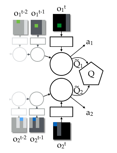
The $q_i$ are learned utilities, not necessarily expected returns from individual rewards. Sunehag et al., Section 3 learn them from a single team reward. Their recurrent networks use local histories; here we use state inputs to isolate the additive argument.

Original Sunehag et al. Figure 2 shows two recurrent agent networks processing local observation histories. Their learned utilities Q-tilde one and Q-tilde two feed a joint Q node, while each network separately selects its agent's action. — **Figure 3. VDN combines utilities into one team value.** Original figure from Sunehag et al. (2017), Value-Decomposition Networks For Cooperative Multi-Agent Learning, Figure 2. Only Figure 2 is excerpted; the neighboring independent-learning Figure 1 is not included. The source utilities are learned from the team reward, not prescribed individual rewards. Full resolution ↗Figure excerpt for discussion; copyright remains with the authors/rightsholder.

Why independent greedy actions maximize the sum

Fix $s$ and let $a_i^*\in\arg\max_{a_i}q_i(s,a_i)$ . For every joint action,

\sum_iq_i(s,a_i) \le\sum_i\max_{u_i}q_i(s,u_i) =\sum_iq_i(s,a_i^*).

Conversely, if one coordinate is not a utility maximizer, replacing it strictly improves the sum. Hence the full sets agree, including ties:

\boxed{ \arg\max_{\boldsymbol a}Q_{\mathrm{tot}}(s,\boldsymbol a) =\prod_i\arg\max_{a_i}q_i(s,a_i). }

Independent maximization therefore recovers a maximum of the fitted additive value. Whether that value can represent the true optimal team value is a separate approximation question.

How one team error trains several utilities

Let $Z=(S,\boldsymbol A,R,S')\sim\mu$ denote a draw from a fixed replay-buffer distribution; condition on the realized buffer. With frozen target parameters $w^-$ , set

\begin{aligned} y(Z)&=R+\gamma\sum_i\max_{u_i}q_{i,w_i^-}(S',u_i),\\ \mathcal L(w)&=\frac12\mathbb E_{Z\sim\mu} \left[\{Q_{\mathrm{tot},w}(S,\boldsymbol A)-y(Z)\}^2\right],\\ \nabla_{w_i}\mathcal L(w) &=\mathbb E_{Z\sim\mu} \left[(Q_{\mathrm{tot},w}-y)\nabla_{w_i}q_{i,w_i}(S,A_i)\right]. \end{aligned}

The continuation term is zero at genuine terminals. The last line uses separate utility parameters and a fixed target; differentiating the square distributes one team prediction error to each utility. This is not a policy-gradient estimator, and replay samples do not have law $\nu_\theta$ in general.

Nor are utilities uniquely identified: adding $c(s)$ to $q_1$ and subtracting it from $q_2$ leaves $Q_{\mathrm{tot}}$ and greedy actions unchanged. A useful value decomposition is not a unique causal attribution of reward.

7. QMIX: a monotonic rather than additive restriction

QMIX replaces the sum with a state-dependent mixing function:

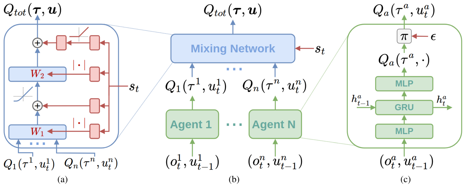
Q_{\mathrm{tot}}(s,\boldsymbol a) =m_s\bigl(q_1(s,a_1),\ldots,q_N(s,a_N)\bigr), \qquad \frac{\partial m_s}{\partial q_i}\ge0.

The mixer is nondecreasing in each utility when the others are fixed. For a differentiable mixer on a box-shaped domain, the displayed derivative condition ensures this property. Nonnegative mixing weights and nondecreasing activations enforce it. Networks called hypernetworks generate those weights from the state. The mixer need not be monotonic in the state. See Rashid et al., Section 4.

Original Rashid et al. Figure 2 shows a mixing network with absolute-value constrained nonnegative weights supplied by state-conditioned hypernetworks, the combination of N agent utilities into Q-total, and a recurrent agent network that produces action utilities from local observations and previous actions. — **Figure 4. QMIX's state-conditioned monotonic mixing network.** Original figure from Rashid et al. (2018), QMIX: Monotonic Value Function Factorisation for Deep Multi-Agent Reinforcement Learning, Figure 2. All three architecture panels are retained. Monotonicity concerns the utility inputs at fixed state, not the state input itself; the source actors use local histories. Full resolution ↗Figure excerpt for discussion; copyright remains with the authors/rightsholder.

Again fix $s$ , so the mixer and its state-conditioned parameters do not change during action comparison. If each $a_i^*$ maximizes $q_i$ , coordinatewise replacement yields

\begin{aligned} m_s(q_1(s,a_1),\ldots,q_N(s,a_N))\\ &\le m_s(q_1(s,a_1^*),q_2(s,a_2),\ldots,q_N(s,a_N))\\ &\le\cdots\le m_s(q_1(s,a_1^*),\ldots,q_N(s,a_N^*)). \end{aligned}

Thus decentralized greedy selection is sufficient:

\boxed{ \prod_i\arg\max_{a_i}q_i(s,a_i) \;\subseteq\;\arg\max_{\boldsymbol a}Q_{\mathrm{tot}}(s,\boldsymbol a). }

With nonstrict monotonicity, set equality need not hold: $m_s(u_1,u_2)=u_1$ ignores agent 2, so even its nongreedy actions can maximize $Q_{\mathrm{tot}}$ . The inclusion above states exactly the greedy guarantee needed here.

More expressive than a sum, but not unrestricted

For two binary actions, consider the team action-value table

M=\begin{pmatrix}1&2\\2&4\end{pmatrix}.

An additive table $M_{ab}=x_a+y_b$ must satisfy $M_{11}-M_{10}-M_{01}+M_{00}=0$ . Here that contrast is $1$ , so VDN cannot represent the table exactly. However, $q_i(0)=1$ , $q_i(1)=2$ , and $m(u_1,u_2)=u_1u_2$ represent it and are monotonic on $[1,2]^2$ . This demonstrates the larger monotonic function class, not exact representation by every finite QMIX network.

Now return to Part 1's coordination table:

C=\begin{pmatrix}2&0\\0&1\end{pmatrix}.

If $q_1(0)>q_1(1)$ , monotonicity forces $C_{00}\ge C_{10}$ and $C_{01}\ge C_{11}$ ; the latter is false. Reversing the utility ordering contradicts the first column. Equal utilities force equal rows. No fixed scalar utility ordering for agent 1 can represent this entire table through a monotonic mixer.

Nevertheless, the optimal joint action $(0,0)$ is perfectly decentralized. Failure to represent all action values does not imply failure to express an optimal joint choice. Monotonic mixing is sufficient, not necessary, for greedy consistency. The original QMIX analysis studies this representational restriction rather than claiming that all cooperative games satisfy it.

8. What each construction preserves

Construction	What is compared or learned?	Established property
Immediate difference reward	One action versus a reference, at fixed state and teammates' actions	Preserves immediate action rankings at that context
COMA	One action versus its policy-weighted alternatives in a joint critic	Preserves the expected on-policy gradient with an exact critic
VDN	Additive utilities fitted to a team value target	Independent utility maxima are exactly the sum's joint maxima
QMIX	Utilities combined by a monotonic mixer	Independent utility maxima give a joint maximum of the fitted value

The first two compare an agent's action with alternatives; the latter two constrain a value representation. None alone proves global convergence or supplies a unique division of team reward. Part 3 examines which information the agents may use during training and execution; Part 4 develops multi-agent actor–critic updates.

References

Foerster, J. N., Farquhar, G., Afouras, T., Nardelli, N., and Whiteson, S. (2018). Counterfactual Multi-Agent Policy Gradients. AAAI. Section 4 defines the counterfactual advantage and gives the baseline cancellation; Figure 1 shows the architecture.
Sunehag, P., Lever, G., Gruslys, A., Czarnecki, W. M., Zambaldi, V., Jaderberg, M., Lanctot, M., Sonnerat, N., Leibo, J. Z., Tuyls, K., and Graepel, T. (2017). Value-Decomposition Networks For Cooperative Multi-Agent Learning. Section 3 of the linked first-version PDF gives the additive construction; Figures 2–3 show the architecture and tasks.
Rashid, T., Samvelyan, M., de Witt, C. S., Farquhar, G., Foerster, J., and Whiteson, S. (2018). QMIX: Monotonic Value Function Factorisation for Deep Multi-Agent Reinforcement Learning. ICML. Sections 3.4–4 explain decentralized greedy selection and monotonic mixing; Figure 2 shows the architecture.

The Bernoulli calculations, delayed-reward counterexample, and small matrix examples above are worked examples for this note, not experimental results from these papers.