Reinforcement Learning, Part i: Foundations and Learning Methods

Reinforcement Learning: i. Foundations and learning methods · ii. Partial observability, offline data, and DTRs.

Reinforcement learning studies how actions affect both immediate rewards and future decisions. We begin with a fully observed Markov decision process, derive the Bellman equations for expected return, and prove why exact value iteration converges. We then distinguish methods by the model, optimization target, and data they use. The setup follows Sutton–Barto, Chapter 3; the contraction argument follows Reinforcement Learning: Theory and Algorithms, Section 1.3.1.

1. A Markov decision process and its assumptions

Let $\mathcal S$ and $\mathcal A$ be nonempty finite state and action sets. At time $t=0,1,\ldots$, the agent observes $S_t\in\mathcal S$, selects $A_t\in\mathcal A$, and receives $R_{t+1}\in\mathbb R$ together with the next state $S_{t+1}$. Fix an ordering of actions to resolve ties.

Write the full available history as

The controlled Markov assumption is an equality of conditional distributions:

Thus the current state and action determine the conditional distribution of the next state and reward; earlier history adds no further information. Writing $p$ without a time index also assumes time-homogeneous dynamics: the transition law does not change with time. Calling an observed variable a state does not establish either assumption.

We use the MDP specification

and assume $|R_{t+1}|\le R_{\max}<\infty$ almost surely under every state–action transition. Here $p(s',dr\mid s,a)$ is a probability kernel on next states and rewards. Its state marginal and conditional reward mean are

For transitions with $P(s'\mid s,a)=0$, the value assigned to $\mathcal R(s,a,s')$ does not affect this sum. The joint kernel defines the reward distribution; $(P,r)$ is sufficient for the expected-return Bellman equations.

Click to enlarge · Scroll sideways on small screens

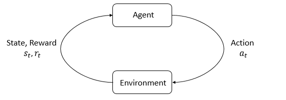
The model need not be known. The MDP describes the environment; a learning algorithm may have to estimate its consequences from sampled transitions. Temporal dependence within a trajectory is allowed. Independent one-step observations are not an MDP assumption.

2. Policies, returns, and the optimization target

A stationary Markov policy is a map $\pi:\mathcal S\to\Delta(\mathcal A)$, where $\Delta(\mathcal A)$ denotes the probability simplex:

The agent samples $A_t\sim\pi(\cdot\mid S_t)$ using fresh randomization. A deterministic policy $d:\mathcal S\to\mathcal A$ is the special case $\pi(a\mid s)=\mathbf1\{a=d(s)\}$. More generally, a policy can depend on time and the full history through $\pi_t(a\mid H_t)$, but not on future information. Such policies are called nonanticipating; we include them in the optimality proof.

Write $\mathbb P_{\rho_0}^{\pi}$ for the trajectory distribution generated by

Expectations $\mathbb E_{\rho_0}^{\pi}$ average over all these draws, with the policy and environment fixed. The shorter $\mathbb E^\pi$ uses this distribution, with any stated conditioning. A policy subscript therefore includes environment randomness, not just sampled actions. For a history-dependent policy $\mu$, replace the action distribution by $\mu_t(\cdot\mid H_t)$. A one-transition expectation at fixed $(s,a)$ instead integrates only $(S',R)\sim p(\cdot\mid s,a)$.

Define the discounted return

Bounded rewards and $\gamma<1$ imply

The return therefore exists absolutely. This bound also justifies the expectation and limit operations below by dominated convergence.

For a stationary Markov policy, define

Here $\mathbb E_s^\pi$ uses the trajectory distribution above with $S_0=s$ fixed, rather than drawn from $\rho_0$. The expectation $\mathbb E_{s,a}^\pi$ also fixes $A_0=a$, then follows $\pi$ for later actions. This defines $Q^\pi(s,a)$ even if $\pi(a\mid s)=0$. On events of positive probability, these definitions agree with the usual conditional expectations.

In $J_{\rho_0}$, the value function $V^\pi$ is fixed. The outer expectation averages only over the initial state $S_0\sim\rho_0$.

These are population value functions, not their fitted estimates. Policy evaluation determines $V^\pi$ or $Q^\pi$ for a fixed policy; control seeks a policy maximizing expected return.

3. Deriving the Bellman expectation equations

First, condition on the initial action. The law of total expectation gives

Next, substitute the return recursion into the action value:

The second equality is the tower property. The third uses both the controlled Markov dynamics and the stationary Markov policy: conditional on $S_1$, the continuation has the same law as a process newly started there. No independence between the immediate reward and next state is needed.

Combining the two identities gives

Alternatively, substituting the action average for $V^\pi(s')$ gives

A matrix form for policy evaluation

Let $m=|\mathcal S|$. Regard $V^\pi,r^\pi\in\mathbb R^m$ as vectors and $P^\pi\in\mathbb R^{m\times m}$ as a transition matrix, with

Then

To justify the inverse, use $\|P^\pi\|_\infty=1$ for the induced matrix norm. The convergent Neumann series gives

The $k$th term is the expected reward $k$ transitions into the future, discounted by $\gamma^k$.

The advantage function is

The advantage therefore measures how an action's expected return differs from the policy's average at that same state.

4. Optimality and the contraction argument

For $U:\mathcal S\to\mathbb R$, define the Bellman operators

Theorem 1. Under the finite-space, bounded-reward, time-homogeneous assumptions in Section 1, $\mathcal T^*$ has a unique fixed point $v$. It equals the optimal value $V^*$ over all nonanticipating policies. A deterministic policy greedy with respect to $v$ is optimal from every starting state.

First, establish the elementary maximum inequality. For real vectors $(x_a),(y_a)$, choose $a_x\in\arg\max_a x_a$. Then

Interchanging $x$ and $y$ yields the absolute-value version. Apply it inside $\mathcal T^*$:

Because transition probabilities are nonnegative and sum to one, their weighted average cannot exceed the largest value difference. Taking the maximum over states proves

Because $\mathbb R^m$ is complete and $\gamma<1$, the Banach fixed-point theorem supplies a unique fixed point $v$. The same averaging argument makes $\mathcal T^\pi$ a contraction, whose fixed point is $V^\pi$.

Next, select the first maximizing action in the fixed ordering:

By construction $\mathcal T^{d_v}v=\mathcal T^*v=v$. Uniqueness of the policy-evaluation fixed point implies $v=V^{d_v}$. In particular $v$ is an attained policy value and $\|v\|_\infty\le R_{\max}/(1-\gamma)$.

Finally, compare it with any history-dependent randomized policy $\mu$. Since a maximum dominates every action mixture, the Markov assumption gives

Repeated substitution and the tower property yield, for every integer $M\ge1$,

The terminal term tends to zero because $v$ is bounded. Dominated convergence therefore gives $v(s)\ge V^\mu(s)$. Together with $v=V^{d_v}$, this proves $v=V^*$ and optimality of $d_v$ even against nonstationary, history-dependent competitors.

Consequently,

The optimal action is $d^*(s)\in\arg\max_a Q^*(s,a)$; a policy and an action are different mathematical objects.

5. Value iteration and a worked example

Starting from any finite vector $V_0$, iterate $V_{k+1}=\mathcal T^*V_k$. Contraction gives

There is also a computable residual bound. Adding and subtracting $\mathcal T^*V_k$, then applying contraction, gives

Input: Finite $\mathcal S,\mathcal A$; known $P,r$; $0\le\gamma<1$; initial $V_0$; iteration count $K\ge1$; fixed action ordering.

Output: Value approximation $V_K$ and a policy $d_K$ greedy with respect to $V_K$.

1. for $k=0,\ldots,K-1$ do
2. for each $s\in\mathcal S$ do
3. Set $U(s)\gets\max_a\{r(s,a)+\gamma\sum_{s'}P(s'\mid s,a)V_k(s')\}$.
4. end for
5. Set $V_{k+1}\gets U$ simultaneously for all states.
6. end for
7. Set $d_K(s)\gets\operatorname{first}\arg\max_a\{r(s,a)+\gamma\sum_{s'}P(s'\mid s,a)V_K(s')\}$.
8. return $(V_K,d_K)$.

This algorithm plans with a known model. Estimating $P$ or approximating its Bellman updates introduces additional errors, so those procedures need more than the exact-iteration theorem.

Immediate reward can favor the wrong action

Take $\mathcal S=\{0,1\}$, actions $\{\mathrm{wait},\mathrm{move}\}$, and $\gamma=0.9$. The transitions and rewards are deterministic:

State 1 gives $V^*(1)=2+0.9V^*(1)=20$. At state 0, the candidate $V^*(0)=18$ satisfies

Thus the fixed point is $(18,20)$ and moving is optimal at state 0. Waiting forever instead gives $1/(1-0.9)=10$ there. Starting value iteration from zero produces

As the updates propagate future rewards back to state 0, moving becomes preferable to the immediately rewarding loop. The example illustrates the convergence established by the fixed-point proof.

6. Classifying learning methods without mixing categories

The original Spinning Up taxonomy places familiar algorithms in a broader map. The table below then separates design choices that can overlap; they are not mutually exclusive branches of one tree. These distinctions also follow the learning/planning discussion in Sutton–Barto and Levine et al., Section 2.1.

Click to enlarge · Scroll sideways on small screens

For example, actor–critic methods can be on-policy or off-policy. Policy optimization can use a learned dynamics model. A neural network is a representation choice, not a new definition of the decision problem.

Sampled value updates

Monte Carlo evaluation uses a realized return as a target. In finite episodes this is the return through termination; an infinite-horizon implementation must truncate or otherwise estimate the tail. One-step temporal-difference evaluation instead uses

For action values, two familiar targets are

A tabular update at the visited pair takes the form

Other entries are unchanged. SARSA uses the next action sampled under its policy. Q-learning instead uses the best estimated continuation action, even when the behavior policy explores. It is therefore an off-policy control method.

Convergence of these sampled updates requires conditions on how often state–action pairs are visited, the learning rates, and any function approximation. The contraction proof for exact Bellman updates does not establish convergence for every sampled implementation.

Direct policy search and actor–critic

For a differentiable stochastic policy $\pi_\theta$, direct policy optimization targets $J_{\rho_0}(\pi_\theta)$. To state the discounted policy-gradient identity, define the normalized state occupancy

Under positive differentiable action probabilities and conditions permitting differentiation under the expectation, the identity is

This is the policy-gradient theorem in Agarwal et al., Theorem 9.4, stated here rather than proved. A Monte Carlo method estimates the return from trajectories; an actor–critic method uses a fitted value function to estimate the policy update. The latter separates an actor $\pi_\theta$ from a critic such as $\widehat Q_w$ or $\widehat V_w$. The policy-gradient note derives the identity and compares these methods in detail.

7. Which assumptions will change next?

The discounted stationary MDP is one baseline, not the definition of every RL problem. A finite horizon allows $\gamma=1$ with bounded rewards and generally requires stage-specific $P_t,r_t,\pi_t,V_t$. A partially observed problem distinguishes the hidden state from the information available to the policy. Offline learning changes access to data, not necessarily the Markov dynamics.

Part ii redefines these settings explicitly and ends with their connection to the history-based DTR formulation.

References

• Richard S. Sutton and Andrew G. Barto. Reinforcement Learning: An Introduction, second edition. Publisher; accessible earlier author draft. The linked draft is an in-progress edition, not the final published text.
• Alekh Agarwal, Kianté Brantley, Nan Jiang, Sham M. Kakade, and Wen Sun. Reinforcement Learning: Theory and Algorithms. Section 1.3.1 gives contraction and value iteration; Theorem 9.4 gives the policy-gradient identity in the linked version.
• Sergey Levine, Aviral Kumar, George Tucker, and Justin Fu (2020). Offline Reinforcement Learning: Tutorial, Review, and Perspectives on Open Problems. Section 2.1 reviews the RL formulation and algorithm families.