


Part 2 examined credit assignment and value factorization; Part 3 established when a centralized critic preserves a local actor's gradient. We now use those results to study the update itself. We derive the team gradient, identify how replay changes it, and account for teammates whose policies have already been updated.
Recap: Differentiating a product policy
With separate agent parameters and independent action draws conditional on joint history , the earlier factorization gives
Here is agent 's local history. Only its own policy factor depends on . This identity supplies each partial gradient below; shared parameters require a sum over the affected factors instead.
1. Differentiate the joint policy
Use Part 3's finite-horizon cooperative model. There are agents, decisions, bounded shared rewards, and . Agent observes its local history , a projection of the joint history . Conditional on , independent private action draws give
Action, observation, state, and reward spaces are finite here. Assume positive, continuously differentiable action probabilities and separate parameter vectors . The initial distribution and environment kernels do not depend on . Writing their product as , the full trajectory law is
This defines . Histories, actions, and rewards in every on-policy expectation below are sampled from this law. Parameters remain fixed while an episode is generated. For recurrent actors, score derivatives include the dependence through their unrolled memory updates. Set
Define exact conditional values on histories of positive probability:
The multi-agent score identity
First, differentiate the finite trajectory sum. The likelihood-ratio identity and product policy give
Next, condition on . Normalization of the local action distribution implies
Rewards before time are measurable with respect to , so their score-weighted expectations vanish. Since , conditioning on then yields
The last equality uses the same zero-score identity to subtract . This is an exact derivative, not a claim that a fitted critic is exact. A physical-state-only critic needs the additional sufficiency conditions discussed in Part 3.
COMA instead subtracts an agent-specific counterfactual baseline. Its cancellation uses : the other agents' actions do not reveal agent 's private action draw once is fixed. The choice changes the estimator, not the team objective.
Shared parameters change the derivative
If every policy uses the same parameter vector , every action factor contributes:
Adding the agents' score contributions is therefore necessary. Averaging them instead rescales the gradient by ; treating all but one shared-parameter actor as fixed changes the derivative. Sharing weights still does not share observations at deployment.
2. Deterministic actors and MADDPG
We now change the model: the trainer observes a finite Markov state, joint actions are continuous, and actors are stationary deterministic maps of fixed local features:
Each is a fixed local feature map. There is no unrecorded actor memory in this specialization. Let , initial law , mean reward , and transitions . Assume bounded rewards and continuous derivatives of on a neighborhood of the actions used. Parameters are separate.
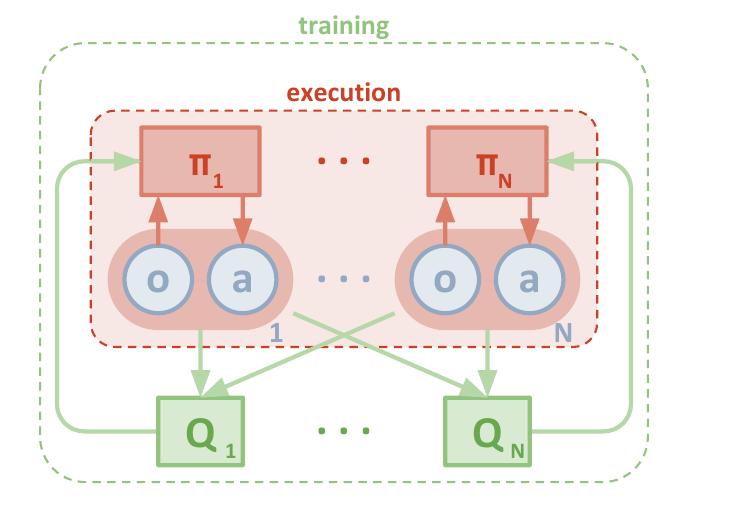
The deterministic value satisfies
Write . Differentiating the Bellman equation gives
Here is an action-by-parameter Jacobian; holds the continuation policy fixed. It already includes the derivative of the immediate reward and transition probabilities. The remaining term differentiates future values.
Because is stochastic and , the Neumann series converges:
Define the normalized discounted state occupancy
Multiplying the series by establishes
This is the multi-agent deterministic gradient under the stated model, obtained by the same Bellman differentiation as Silver et al., Theorem 1. All agents' actions inside the exact critic are their current actions.
Replay changes both the state law and teammates' actions
Multi-agent deep deterministic policy gradient (MADDPG) uses replay and fitted centralized critics. Following Lowe et al., Section 4.1, let denote a transition drawn from a fixed replay buffer. A team-critic version uses
Target parameters are frozen during this regression; terminal transitions use zero continuation. The paper also allows different rewards and critics for different agents. Its replay-based actor update, specialized to a team reward, has direction
Relative to the exact gradient, this direction uses a fitted critic in place of , replay states in place of , and recorded teammate actions in place of their current actions. A learning-rate rescaling cannot correct these changes. Silver et al., Equation 15 likewise treats its off-policy direction as an approximation.
For example, consider one decision with . At current actions ,
The recorded teammate action therefore reverses this derivative even with an exact critic. The discrepancy comes from which joint action is evaluated, not from critic estimation.
To isolate the state-law issue, let be replay's state marginal, with wherever . An exact change of measure gives
This identity still requires the exact evaluated at the agents' current actions. It does not tell us the required state-visitation ratio. Nor does it resolve missing action coverage or make an ordinary replay update an exact on-policy gradient.
3. Local clipping is not joint policy control
Return to the finite-horizon stochastic model in Section 1. Freeze an old product policy and consider a candidate , both positive. Choose . At fixed define
For any function of the joint action, the conditional change of measure is
Even if every actual local ratio were restricted to , the joint ratio would only satisfy
With ten agents and , this interval is approximately . These extremes are attainable at particular joint actions: ten Bernoulli policies changing from probability to give ratios at all ones and at all zeros.
At a fixed history, KL divergence also accumulates across agents. Expanding the logarithm and summing out the other actions gives
PPO clipping is weaker than imposing either displayed restriction: it clips a branch of an objective, not the policy probabilities themselves.
MAPPO's local clipped objective
Let be a frozen team-advantage estimate from an old-policy batch. A per-agent PPO objective is
At , with an exact advantage and separate parameters, its derivative equals agent 's team gradient. For a finite change, it changes only one action factor while retaining the old trajectory law. Concurrently maximizing these local objectives does not make them an exact joint objective for the updated team.
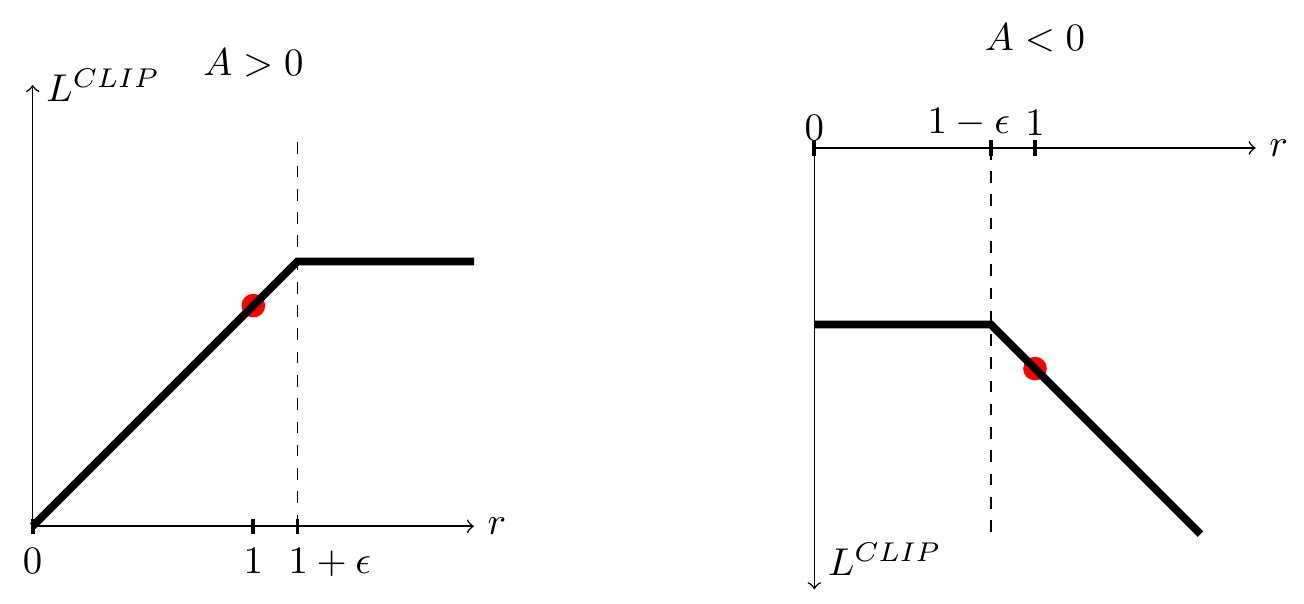
With , the clipped term is flat once . A flat objective branch supplies no hard constraint preventing a larger ratio, particularly when parameters affect many samples.
Multi-agent PPO (MAPPO) combines PPO-style local actors with centralized value inputs. Its homogeneous-agent implementations often share parameters and sum agents' clipped terms. Parameter sharing is an implementation choice, not the definition of CTDE or a requirement of every multi-agent PPO method.
One common advantage estimate is generalized advantage estimation. For a frozen history-value predictor , with and ,
All terms are evaluated on , with the fitted predictor held fixed. The earlier GAE derivation explains the bias–variance tradeoff. A state-only predictor in a partially observed problem needs the qualifications from Part 3; the formula alone does not establish an unbiased history advantage.

These are the authors' SMAC ablations, not results produced here. The same controls both policy and value clipping, so the curves do not isolate the effect of policy clipping. They illustrate practical sensitivity, not a universal optimal or an improvement theorem.
4. Derive the performance-difference identity
To compare two complete policy updates, we need their difference in expected return rather than only a local derivative. Write for the old policy's history values and set . Once is fixed, the environment's next-step law is the same under both policies. Consequently,
Multiply by and sum. Adjacent value terms cancel, the terminal term is zero, and the initial history law is unchanged:
This is an exact finite-horizon identity. The expectation uses candidate-policy histories, not old-policy histories. Since policy probabilities are positive and the environment law is common, the prefix likelihood ratio
changes the old law of to the new law. Therefore an equivalent expression is
Using only changes the current action distribution but still averages over histories from the old policy. This surrogate has the correct first derivative at . At that point, derivatives of the earlier ratios multiply an old-policy conditional advantage with mean zero, so those terms vanish. For a finite update, however, the surrogate need not equal the true change in performance. Trust-region methods therefore need an argument controlling policy change, not just the likelihood-ratio identity.
5. Account for earlier agents' updates
Fix a time , history , and ordering . Suppress temporarily. For an action prefix , average over the remaining old-policy actions:
The endpoints are and . Define an ordered incremental advantage
The letter distinguishes this quantity from the joint advantage . The differences telescope:
Moreover, averaging over its last action under the old policy gives zero at every fixed prefix:
These are the telescoping and marginalization identities behind Kuba et al., Lemma 1. They do not assume additive utilities as in VDN or monotonic mixing as in QMIX. The history-based, finite-horizon version here applies the same algebra separately at each .
Rewrite the incremental improvement using one joint critic
Suppose agents have already selected new policies. Freeze those policies while updating . Define
and the conditional expected increment
First, integrate the unupdated suffix under its old policy. Changing measure for the prefix then gives
The shorthand expectations on the right use exactly the prefix laws in the definition of , with fixed. Subtract the equations. The constant also cancels because . Hence
This is the importance-weight identity in Kuba et al., Proposition 2, with histories replacing states. It uses one joint advantage; separate fitted prefix critics are unnecessary. Dropping would evaluate the current agent against old teammates rather than those already updated.
A sufficient improvement condition
Averaging the telescoping decomposition under the complete candidate policy gives
Therefore, if for every and every candidate-reachable history, the performance-difference identity proves . This is a pointwise sufficient condition. Improving an empirical average over old histories does not establish it.
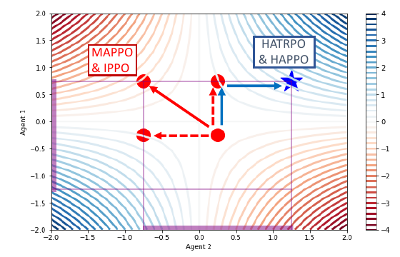
The source's one-state example shows why update order matters. Sample independently for , with means fixed during sampling. Then .
Start from and allow each mean to change by at most one. If both agents optimize against the other's old mean, they choose and reduce return from to . If the first mean changes to before the second agent optimizes, the new pair is and return is . For unit-variance Gaussians, a unit mean displacement has KL divergence , as in the plotted trust regions. This one-decision Gaussian example is separate from our finite-action theorem assumptions.
6. HAPPO-style sequential clipped updates
Heterogeneous-agent proximal policy optimization (HAPPO) uses the sequential correction without requiring shared actor parameters. Replace the exact advantage with a frozen estimate and use the old trajectory batch. The actor at position maximizes
Earlier actors' ratios are fixed during this maximization. Since , multiplying outside the minimum is equivalent to multiplying both branches inside it. The constant from the incremental-improvement identity has zero derivative with respect to the current actor, so it can be omitted. This is the sequential clipped construction of HAPPO, Section 4.2.
Input: Old local actors ; an on-policy batch ; frozen estimates ; clipping width ; an ordering independent of the batch.
Output: Updated local actors .
- Store old action log probabilities for every agent and decision in .
- Initialize for all agents.
- for do
- Compute and freeze on the batch.
- for each optimizer iteration for actor do
- Compute relative to its stored old action probabilities.
- Ascend the empirical , averaging the displayed weighted sum over the episodes; hold all other actors and fixed.
- end for
- Freeze the resulting before proceeding to the next agent.
- end for
- Deploy each updated actor using only its own available history.
This is a simplified actor-update pass, not the paper's complete training procedure. Critic fitting, normalization, learning-rate schedules, and fresh data collection require separate choices. Once the batch and fitted advantages are fixed, the displayed objective is a criterion to optimize on those data. It is not an unbiased estimate of the true improvement after a finite update. Sequential parameter updates also do not require agents to act sequentially at deployment.
Kuba et al.'s Theorem 2 proves monotonic improvement for their ideal policy-iteration algorithm with exact advantages, exact optimization, and a prescribed worst-state KL penalty under their assumptions. Practical HAPPO uses a clipped approximation. Neither that theorem nor the pointwise argument above automatically guarantees improvement for this finite-sample pseudocode.
7. What gradient ascent does and does not guarantee
For separate actors sharing , concatenating their exact partial gradients gives . For a step length , suppose is -Lipschitz along the update segment. The fundamental theorem of calculus gives
Thus a sufficiently small exact joint-gradient update is an ascent step. This statement assumes a common objective, exact gradients, and a suitable step size. It does not prove global optimality, improvement for arbitrary independent surrogate maximizers, or improvement for replay-based approximate gradients.
Different rewards change the problem further. In the one-decision zero-sum game , , with , simultaneous gradient flow in the interior is
For any initial radius in , the parameters cycle inside the action box instead of approaching the Nash equilibrium . There is no shared ascent objective here. A policy-gradient formula alone is not a convergence theorem for a game.
| Update | Main derivative or surrogate | What needs attention |
|---|---|---|
| COMA | Stochastic score times a counterfactual advantage | Baseline cancellation and critic accuracy |
| MADDPG | Action derivative through a deterministic actor | Replay state law, teammate actions, and critic error |
| MAPPO | Local clipped ratios with centralized value estimates | Joint policy change, shared parameters, and history sufficiency |
| HAPPO | Sequential clipped ratios weighted by earlier updates | Frozen prefix ratios and the gap between ideal guarantees and practical clipping |
The four MARL notes now connect the game model to the learning procedure: Part 2 assigns credit, Part 3 checks the critic's information, and this note identifies the objective and sampling distribution behind each actor update.
References
- Silver, D., Lever, G., Heess, N., Degris, T., Wierstra, D., and Riedmiller, M. (2014). Deterministic Policy Gradient Algorithms. ICML. Theorem 1 gives the deterministic gradient; Equation 15 identifies an approximate off-policy update.
- Lowe, R., Wu, Y., Tamar, A., Harb, J., Abbeel, P., and Mordatch, I. (2017). Multi-Agent Actor-Critic for Mixed Cooperative-Competitive Environments. NeurIPS. Section 4.1 gives the centralized deterministic critics and replay-based actor updates; Figure 1 is reproduced above.
- Foerster, J., Farquhar, G., Afouras, T., Nardelli, N., and Whiteson, S. (2018). Counterfactual Multi-Agent Policy Gradients. AAAI. The counterfactual baseline is derived in Part 2 of this series.
- Schulman, J., Wolski, F., Dhariwal, P., Radford, A., and Klimov, O. (2017). Proximal Policy Optimization Algorithms. Section 3 and Figure 1 explain the clipped surrogate.
- Yu, C., Velu, A., Vinitsky, E., Gao, J., Wang, Y., Bayen, A., and Wu, Y. (2022). The Surprising Effectiveness of PPO in Cooperative Multi-Agent Games. NeurIPS, Datasets and Benchmarks. Sections 3 and 5 describe MAPPO and its implementation study; Figure 7 reports the clipping ablation.
- Kuba, J. G., Chen, R., Wen, M., Wen, Y., Sun, F., Wang, J., and Yang, Y. (2022). Trust Region Policy Optimisation in Multi-Agent Reinforcement Learning. ICLR. Lemma 1, Proposition 2, and Section 4.2 motivate the sequential derivation; Theorem 2 concerns the ideal KL-penalized algorithm, not an unconditional guarantee for clipped HAPPO.
The finite-horizon history derivations, replay-action numerical example, and gradient-flow calculation are worked explanations for this note, not new experimental results. Source figures retain their original plots and attribution.