Policy Gradients in Reinforcement Learning

The RL foundations note evaluates a fixed policy through its Bellman equation. To improve a parameterized policy, we now differentiate that value with respect to its parameters. After proving the discounted policy-gradient theorem, we examine how algorithms estimate the gradient, control the update, and change the objective.

Recap: The Bellman inverse used in the proof

For a stationary policy in a finite discounted MDP, policy evaluation gives

Here $P^\pi$ is the policy's state-transition matrix and $r^\pi$ its expected reward vector. The series converges for $\gamma<1$. We use this inverse to propagate a policy change through future state visits.

1. One gradient, several algorithmic choices

We begin with a finite-state, finite-action, time-homogeneous Markov decision process. The environment's transition probabilities $P(s'\mid s,a)$ and expected immediate rewards $r(s,a)$ do not depend on the policy parameter. Assume bounded rewards, a fixed initial distribution $\rho_0$, and $0\le\gamma<1$.

Let $\pi_\theta(a\mid s)>0$ be a continuously differentiable stationary policy, with $\theta$ in an open subset of $\mathbb R^p$. Define

The normalized discounted state distribution and state–action distribution are

Write $\mathbb E_{\nu_\theta}=\mathbb E_{(S,A)\sim\nu_\theta}$: first draw $S\sim d_\theta$, then $A\mid S\sim\pi_\theta(\cdot\mid S)$. This distribution weights state visits across time by their discount factors. It is not the distribution at a single time or an arbitrary distribution sampled from stored experience. Define the policy score $\psi_\theta(s,a)=\nabla_\theta\log\pi_\theta(a\mid s)$, which measures how the log action probability changes with the policy parameters.

Let $P_{\pi_\theta}$ be the trajectory distribution generated by $S_0\sim\rho_0$, actions from $\pi_\theta(\cdot\mid S_t)$, and next states/rewards from the fixed environment kernel $p(\cdot\mid S_t,A_t)$ of the foundations note. We write $\mathbb E_{\pi_\theta}=\mathbb E_{\tau\sim P_{\pi_\theta}}$ for trajectory expectations, including their conditional versions. The notation $\mathbb E_s^{\pi_\theta}$ fixes $S_0=s$ instead of drawing it from $\rho_0$. All these averages hold $\theta$ fixed; differentiating them later accounts for their dependence on $\theta$.

Click to enlarge · Scroll sideways on small screens

The methods below change different parts of policy optimization. REINFORCE and actor–critic estimate the gradient differently. Natural gradients change how we measure the size of a policy update, while TRPO and PPO change the update criterion. Deterministic gradients require different policy and action-space assumptions. Entropy regularization changes the objective to also reward randomness in action choices. An algorithm can combine several of these choices.

2. The discounted policy-gradient theorem

Theorem 1. Under the assumptions above,

This is the discounted start-distribution form of the policy-gradient theorem in Sutton et al. (1999), Theorem 1. The factor $1/(1-\gamma)$ appears because $d_\theta$ is normalized.

First, differentiate the Bellman identity $V^\theta(s)=\sum_a\pi_\theta(a\mid s)Q^\theta(s,a)$. Put

Since the environment is fixed, $\nabla_\theta Q^\theta(s,a)=\gamma\sum_{s'}P(s'\mid s,a)u_\theta(s')$. The product rule gives

where $P_\theta(s,s')=\sum_a\pi_\theta(a\mid s)P(s'\mid s,a)$. The inverse exists by the Neumann-series argument. Applied coordinatewise to $u_\theta$,

Next, average over the initial distribution:

The final equality uses $\nabla\pi_\theta=\pi_\theta\nabla\log\pi_\theta$. Differentiability follows directly from the finite-dimensional inverse formula for $V^\theta$; the convergent series represents that derivative. We have not discarded the effect of changing state visitation: the inverse propagates it through every future transition.

Finally, for each state,

Thus any finite state-only baseline $b(s)$ has $\mathbb E_{\nu_\theta}[\psi_\theta b(S)]=0$. Choosing $b=V^\theta$ proves the advantage form. $\square$

3. REINFORCE: Use sampled returns

The likelihood-ratio construction leads to the Monte Carlo estimator

The batch $\mathcal B=(\tau_1,\ldots,\tau_n)\sim P_{\pi_\theta}^{\otimes n}$ consists of independent current-policy trajectories. Conditional on $(S_t,A_t)$, the return under $P_{\pi_\theta}$ has mean $Q^\theta(S_t,A_t)$. The tower property and the mean-zero score therefore give $\mathbb E_{\mathcal B\sim P_{\pi_\theta}^{\otimes n}}[\widehat g_{\mathrm{MC}}]=\nabla J$. This is the return-based policy-gradient construction associated with Williams's REINFORCE algorithms.

The identity uses full returns, or returns through genuine terminal states in episodic problems. An arbitrary rollout cutoff without its continuation value changes the target. The baseline must be held fixed relative to the trajectory used for this unbiasedness argument; estimating it from those same outcomes needs an additional argument.

Which baseline minimizes variance?

Fix a state $s$ and consider the vector contribution $X_b=\psi_\theta(s,A)(G-b)$. In this subsection, $(A,G)\mid S=s$ is drawn by sampling $A\sim\pi_\theta(\cdot\mid s)$ and then the discounted continuation return from the environment and policy. The conditional expectations below use that distribution, with $s,\theta,b$ fixed. Its conditional mean is independent of $b$. Hence minimizing the trace of its conditional covariance is equivalent to minimizing

Differentiate this scalar quadratic in $b$. If its denominator is positive, the minimizer is

If the denominator is zero, the score is zero almost surely at that state and every baseline is equivalent. This is a variance optimum for a single conditional score contribution, not automatically for the sum of correlated contributions in an episode. In general $b^*(s)\ne V^\theta(s)$.

For one decision, let $A\sim\operatorname{Bernoulli}(p)$ with $p=\sigma(\theta)=0.2$, reward $Y=A\in\{0,1\}$, and score $\psi=A-p$. Only $A$ is random, so

The value baseline $b=0.2$ reduces variance from $0.1024$ to $0.0576$; $b^*=0.8$ makes both possible gradient contributions equal to $0.16$. This is an exact illustrative calculation, not an empirical benchmark.

Scroll horizontally to inspect the full figure →

4. Actor–critic and generalized advantage estimation

An actor–critic method learns a value function alongside the policy. With an approximate action value $Q_w$, replacing $Q^\theta$ in the theorem gives

Consequently Cauchy–Schwarz yields

A critic can introduce bias; a small prediction error and an exactly unbiased gradient are different properties. Sutton et al., Theorem 2 gives an important exception. For a compatible advantage critic $f_w(s,a)=w^\top\psi_\theta(s,a)$, minimize the population loss

Stationarity in $w$ gives

Here the fitted critic gives the exact gradient because the mean product of its residual and the policy score is zero. This is the orthogonality established by the preceding equation. The result requires the displayed population regression, with policy parameters and the sampling distribution fixed. It does not hold for an arbitrary neural critic.

From TD residuals to GAE

For a bounded state-value approximation $V_w$, define its temporal-difference residual

Here $w$ and $\theta$ are fixed. Conditional on $(S_t,A_t)$, $\delta_t^w$ varies through $(S_{t+1},R_{t+1})\sim p(\cdot\mid S_t,A_t)$. If $V_w=V^\theta$, the Bellman equation gives $\mathbb E_{\pi_\theta}[\delta_t^w\mid S_t,A_t]=A^\theta(S_t,A_t)$. To incorporate more subsequent rewards, sum $k$ residuals:

The intermediate value terms cancel. Generalized advantage estimation (GAE) mixes these horizons. For $0\le\lambda<1$,

Bounded rewards and $V_w$ justify the rearrangement by absolute convergence. Here $\lambda$ is a trace parameter, unrelated to the kernel noise scale in the earlier article.

Scroll horizontally to inspect the full figure →

At $\lambda=0$, the estimator is one TD residual. At $\lambda=1$, the residual series telescopes to $G_t-V_w(S_t)$ because $\gamma^kV_w(S_{t+k})\to0$. The latter gives an unbiased score-gradient contribution for any fixed state-only $V_w$; its conditional mean need not equal the true advantage unless $V_w=V^\theta$.

If $V_w=V^\theta$, all later residuals have zero conditional mean after averaging over their policy-selected actions. Thus every $\lambda\in[0,1]$ yields the correct conditional advantage. With an imperfect critic, $\lambda<1$ can introduce bias while changing variance. No universal monotone ordering of variances is implied. Unlike the GAE paper's discussion of discounting an undiscounted objective, our target is explicitly $J$ with the fixed discount $\gamma$.

5. Natural gradients: Measure changes in policies

Ordinary ascent uses the direction $g=\nabla J$ in parameter coordinates. Natural policy gradients instead use a local metric on action distributions. Following Kakade's natural policy gradient, define

For this derivation, assume the policy is twice continuously differentiable and $F_\theta$ is positive definite. We measure the change between action distributions using Kullback–Leibler (KL) divergence. Holding the reference state distribution $d_\theta$ fixed, expand its average:

The linear term vanishes by the mean-zero score. For the Hessian, differentiating $\sum_a\pi_\theta(a\mid s)=1$ twice gives

The KL expansion measures policy change by a quadratic form. We therefore compare candidate update directions under the local constraint

For $g\ne0$ and $\delta>0$, the Lagrangian equation $g=\eta F_\theta\Delta$ and an active constraint give

The natural-gradient direction is $F_\theta^{-1}g$. For $g=0$, choose $\Delta=0$. Redundant parameterizations, including unrestricted softmax logits, can make $F_\theta$ singular; an ordinary inverse is then unavailable. Damping or an appropriate pseudoinverse requires a modified treatment, not the positive-definite calculation above.

Scroll horizontally to inspect the full figure →

The compatible-critic normal equations from the preceding section are $F_\theta w=(1-\gamma)g$. When the inverse exists, its coefficients therefore point in the natural-gradient direction. Kakade's original presentation uses an average-reward distribution; the factor here follows from our normalized discounted convention.

6. TRPO and PPO: Change the update criterion

Let $\pi$ be the old policy and $\pi'$ a candidate. The performance-difference identity is

To establish it, take a trajectory under $\pi'$. Conditional expectation of $R_{t+1}+\gamma V^\pi(S_{t+1})-V^\pi(S_t)$ given $(S_t,A_t)$ equals $A^\pi(S_t,A_t)$. Discount and sum through time $m-1$:

Bounded values make the final term vanish as $m\to\infty$. The definition of normalized occupancy then gives the identity. This is the starting point of Schulman et al.'s TRPO analysis.

A local surrogate and a trust region

Replace the candidate state distribution by the old one to define

At $\pi'=\pi$, it equals $J(\pi)$ and has the same parameter gradient as $J$. For the derivative, any change in $d_{\pi'}$ multiplies $\sum_a\pi(a\mid s)A^\pi(s,a)=0$ at the old policy, leaving exactly the policy-gradient term. Away from the old policy the two objectives need not agree.

Practical trust region policy optimization (TRPO) approximately maximizes the sample surrogate subject to an average KL constraint. It uses a linear approximation to the objective and a quadratic approximation to KL, giving the natural-gradient calculation above. It then checks the proposed update.

The paper's theoretical improvement bound instead controls the largest divergence over all states. Replacing that quantity by a sampled average KL is a practical approximation. It does not guarantee that every update improves the true return.

PPO's clipped surrogate

Proximal policy optimization (PPO) uses the action ratio $\varrho_\theta(s,a)=\pi_\theta(a\mid s)/\pi_{\mathrm{old}}(a\mid s)$ and a fixed advantage estimate $\widehat A$. For $0<\epsilon<1$, its clipped term is

The two signs of advantage give different plateaus:

The sampled objective averages these terms. The original PPO paper's Figure 1 shows the sign-dependent clipping directly.

Click to enlarge · Scroll sideways on small screens

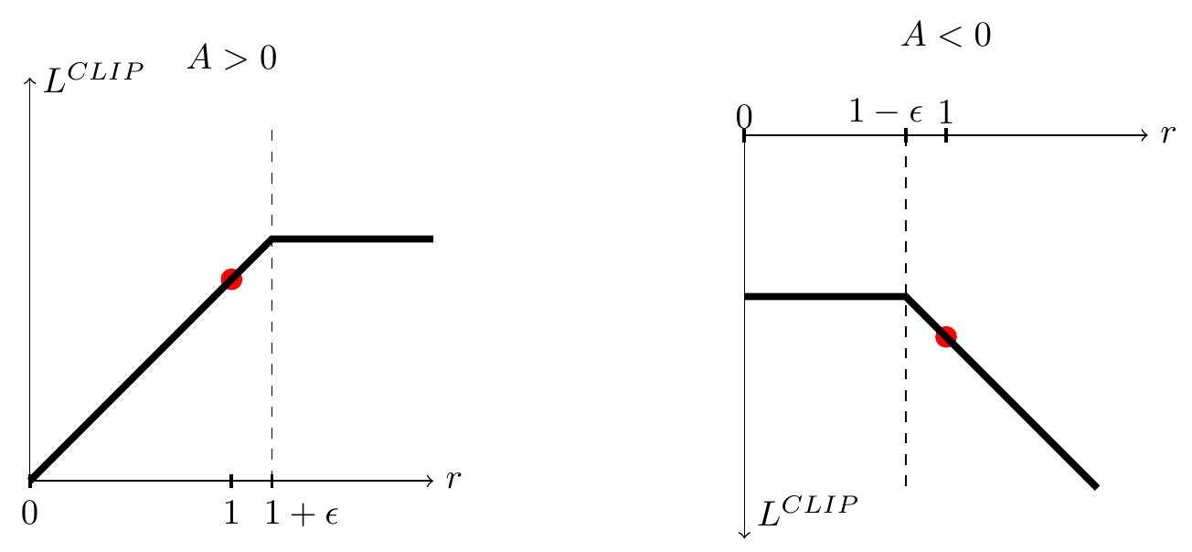
At ratio one, its derivative matches the ordinary surrogate's derivative. Clipping removes an individual sample's incentive to increase a favorable ratio beyond its plateau. It does not constrain every ratio to the clipping interval, clip the policy's action probabilities, or establish a hard KL bound. This is why PPO's objective and TRPO's constrained update remain distinct.

7. Deterministic and reparameterized policy gradients

We now change assumptions. Keep finite states and $\gamma<1$, but let actions range over an open subset of $\mathbb R^m$. A deterministic policy $\mu_\theta(s)$ takes values in that set. Assume $\mu_\theta$, the expected reward, and transition probabilities are continuously differentiable in the relevant parameters/actions; rewards remain bounded. These finite-state conditions make the Bellman inverse differentiable.

Let $D_\theta\mu_\theta(s)\in\mathbb R^{m\times p}$ be the action Jacobian. Differentiating the deterministic Bellman equation gives

Differentiating the current action produces the first term. The second accounts for changes in future actions, which we propagate through the Bellman inverse as in Theorem 1:

This is a finite-state version of Silver et al.'s deterministic policy-gradient theorem. There is no $\log\pi_\theta$ for a point-mass policy. A deterministic argmax over categorical action labels is not the differentiable continuous-action map required here.

The gradient passes through the action input of a critic, not through the unknown physical environment. Exploration may use a separate stochastic behavior policy. Replacing $d_{\mu_\theta}$ by an uncorrected replay-state distribution does not preserve this exact start-distribution gradient in general; Silver et al. explicitly distinguish their off-policy approximation.

Click to enlarge · Scroll sideways on small screens

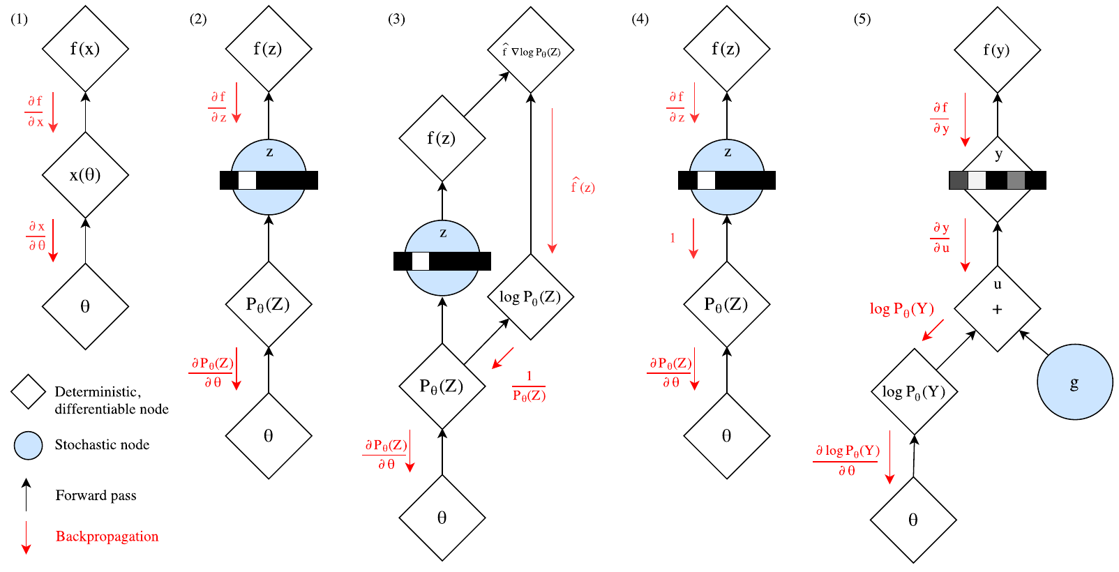
A stochastic policy can also admit a pathwise gradient: write $A=g_\theta(s,\xi)$ with parameter-independent noise $\xi$. The policy remains stochastic because $\xi$ varies. This differs from both a deterministic actor and a score-function estimator; Jang et al., Figure 2 illustrates the distinction between differentiating a likelihood and differentiating a sample transformation.

8. Entropy-regularized stochastic actors

Soft actor–critic (SAC) combines a stochastic actor, a critic, off-policy training, and an entropy-regularized objective. It is not another name for natural gradients or PPO. In the finite-action setting, the discounted maximum-entropy target is

The conditional mean of $-\log\pi(A_t\mid S_t)$ is the policy's entropy. To isolate one policy-improvement subproblem, hold a soft critic $Q_w$ fixed at a state and consider the actor loss

For finite actions, define $Z_w(s)=\sum_a\exp\{Q_w(s,a)/\alpha\}$ and $p_w(a\mid s)=\exp\{Q_w(s,a)/\alpha\}/Z_w(s)$. Direct substitution gives

Nonnegativity of KL shows that unrestricted minimization chooses $\pi=p_w$. This is the finite-action counterpart of the soft policy-improvement projection in Haarnoja et al., Sections 4.1–4.2. Its critic is entropy-regularized; simply adding entropy to an update using an unchanged ordinary critic is not a derivation of the full SAC algorithm.

Scroll horizontally to inspect the full figure →

For continuous actions and a reparameterizable actor, let $d_{\mathcal D}$ be the fixed distribution used to draw replay states (for uniform sampling from a buffer of $m$ states, $d_{\mathcal D}=m^{-1}\sum_{j=1}^m\delta_{s_j}$). Draw $S\sim d_{\mathcal D}$ and independently $\xi\sim q_\xi$, a specified parameter-independent noise distribution, with $g_\theta(s,\xi)\sim\pi_\theta(\cdot\mid s)$. Hold the critic, buffer, and $q_\xi$ fixed. The SAC-style actor objective is

Assuming differentiability and an integrable local bound that permits differentiation under the expectation, its pathwise derivative is

The log density changes in two ways: its parameters change directly, and its action input changes through the sampled action. The total derivative includes both terms. This gives the actor-loss derivative in the SAC paper, Equations (12)–(13), with $\alpha$ written explicitly. Averaging this actor loss over stored states does not generally give the ordinary on-policy gradient of $J$.

9. An on-policy actor–critic template

For a compact algorithm, specialize to episodes that terminate after $T$ decisions, include decision time in the state, and set terminal value to zero. The continuing formulation above then represents the same problem with absorbing zero rewards after termination. Take unconstrained policy parameters in $\mathbb R^p$.

Input: Initial policy parameters $\theta$ and critic parameters $w$; $0\le\gamma<1$; $0\le\lambda\le1$; iterations $B\ge1$; $n\ge1$ episodes per iteration; positive actor learning rates $\eta_r$.

Output: Fitted stochastic policy $\pi_\theta$.

1. for $r=0,\ldots,B-1$ do
2. Freeze the current actor $\theta_{\mathrm{old}}\gets\theta$ and critic $w_{\mathrm{old}}\gets w$.
3. Collect $n$ independent complete episodes under $\pi_{\theta_{\mathrm{old}}}$.
4. for each episode $i$ do
5. Set $\widehat A_{Ti}\gets0$, $G_{Ti}\gets0$, and $V_{w_{\mathrm{old}}}(S_{Ti})\gets0$ at the terminal state.
6. for $t=T-1,\ldots,0$ do
7. Set $\delta_{ti}\gets R_{t+1,i}+\gamma V_{w_{\mathrm{old}}}(S_{t+1,i})-V_{w_{\mathrm{old}}}(S_{ti})$.
8. Set $\widehat A_{ti}\gets\delta_{ti}+\gamma\lambda\widehat A_{t+1,i}$ and $G_{ti}\gets R_{t+1,i}+\gamma G_{t+1,i}$.
9. end for
10. end for
11. Compute $\widehat g\gets n^{-1}\sum_i\sum_{t=0}^{T-1}\gamma^t\nabla_\theta\log\pi_{\theta_{\mathrm{old}}}(A_{ti}\mid S_{ti})\widehat A_{ti}$, holding all advantages fixed.
12. Update $\theta\gets\theta_{\mathrm{old}}+\eta_r\widehat g$.
13. Fit $V_w$ to the fixed targets $\{(S_{ti},G_{ti})\}$, retaining value zero at terminal states.
14. end for
15. return $\pi_\theta$.

This is a simplified methodological template, not a reproduction of TRPO, PPO, or SAC. Advantages use the critic frozen before the current batch. For $\lambda<1$, critic approximation can bias the actor update; no general global-convergence guarantee is asserted. The factor $\gamma^t$ retains the start-distribution discounted objective used in this article.

10. Connect the method to its assumptions

The offline-learning article separates data access from policy type. Neither an actor–critic label nor a single action-probability ratio automatically corrects the state distribution of arbitrary logged data.

References

• Ronald J. Williams (1992). Simple Statistical Gradient-Following Algorithms for Connectionist Reinforcement Learning. Machine Learning, 8, 229–256. Open paper. REINFORCE and likelihood-ratio updates.
• Richard S. Sutton, David McAllester, Satinder Singh, and Yishay Mansour (1999). Policy Gradient Methods for Reinforcement Learning with Function Approximation. NeurIPS. Theorems 1–2: policy gradients and compatible critics.
• Sham Kakade (2001). A Natural Policy Gradient. NeurIPS. Fisher geometry and compatible function approximation. We use a normalized discounted variant rather than the paper's average-reward convention.
• John Schulman, Philipp Moritz, Sergey Levine, Michael Jordan, and Pieter Abbeel (2016). High-Dimensional Continuous Control Using Generalized Advantage Estimation. ICLR. Section 3, Equations (14)–(18).
• John Schulman, Sergey Levine, Philipp Moritz, Michael Jordan, and Pieter Abbeel (2015). Trust Region Policy Optimization. ICML. Performance differences, surrogate objectives, and theoretical versus practical divergence control.
• John Schulman, Filip Wolski, Prafulla Dhariwal, Alec Radford, and Oleg Klimov (2017). Proximal Policy Optimization Algorithms. Section 3 and Figure 1.
• David Silver, Guy Lever, Nicolas Heess, Thomas Degris, Daan Wierstra, and Martin Riedmiller (2014). Deterministic Policy Gradient Algorithms. ICML. Theorem 1 and the distinction between on-policy identities and off-policy approximations.
• Tuomas Haarnoja, Aurick Zhou, Pieter Abbeel, and Sergey Levine (2018). Soft Actor-Critic: Off-Policy Maximum Entropy Deep Reinforcement Learning with a Stochastic Actor. ICML. Soft policy improvement and the reparameterized actor loss.
• Eric Jang, Shixiang Gu, and Ben Poole (2017). Categorical Reparameterization with Gumbel-Softmax. ICLR. The reproduced Figure 2 distinguishes several gradient estimators; its final panel is the paper's categorical relaxation, not a continuous-action SAC diagram.