


A language model stores earlier tokens' key and value vectors so it can reuse them when generating the next token. This stored information, called the KV cache, grows with context length and network depth. We derive its storage cost, then examine how DeepSeek-V4.1-Flash lets several layers share cached representations while computing different attention outputs.
The Two Minute Papers video motivates this question. We develop the attention, GPT, and cache-sharing calculations from primary papers rather than the video's benchmark comparisons.
Recap: A language model is a conditional token distribution
As in the alignment note, we factor the joint distribution of tokens in a finite vocabulary into conditional probabilities:
During generation, , with trained parameters fixed; the empty prefix uses a start token. Although the token is sampled, its probabilities are deterministic given the prefix when dropout is disabled. We examine which intermediate computations can therefore be cached.
1. Attention reads a set of vectors
Attention combines information across token positions. Let contain one row per token. For one head, we project these rows using learned matrices and :
The query scores key at position ; the resulting attention weight multiplies value . Vaswani et al., Section 3.2 define this operation as scaled dot-product attention:
For causal attention, we set if and otherwise, giving for future positions. The weights are computed from the query and keys, without an additional random draw.
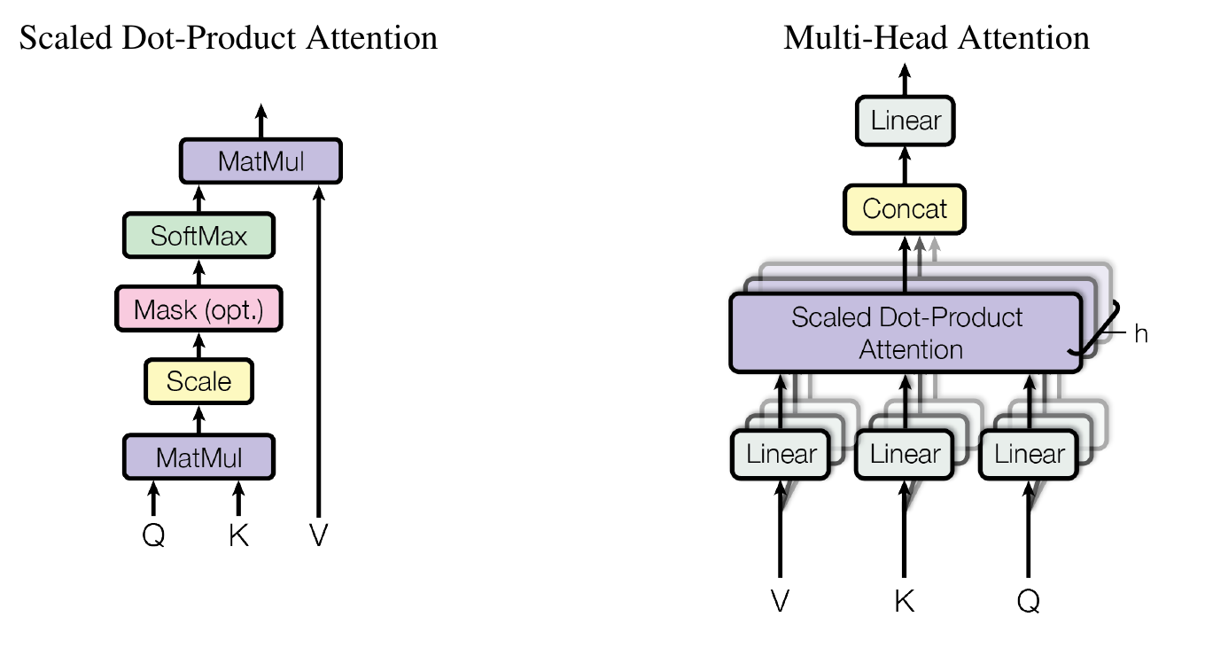
Why divide by the square root?
To examine the score variance, let . Under this auxiliary law,
Dividing by the square root keeps this variance constant as the head dimension grows. This calculation explains the scaling convention without assuming that trained queries and keys are independent Gaussians.
Multi-head attention combines heads' separate outputs :
Different query projections allow these heads to weight the same positions differently.
2. From the Transformer decoder to GPT
The original Transformer encodes an input sequence and decodes an output sequence. Within the decoder, masked self-attention combines previous output positions, whereas cross-attention reads the encoder states.
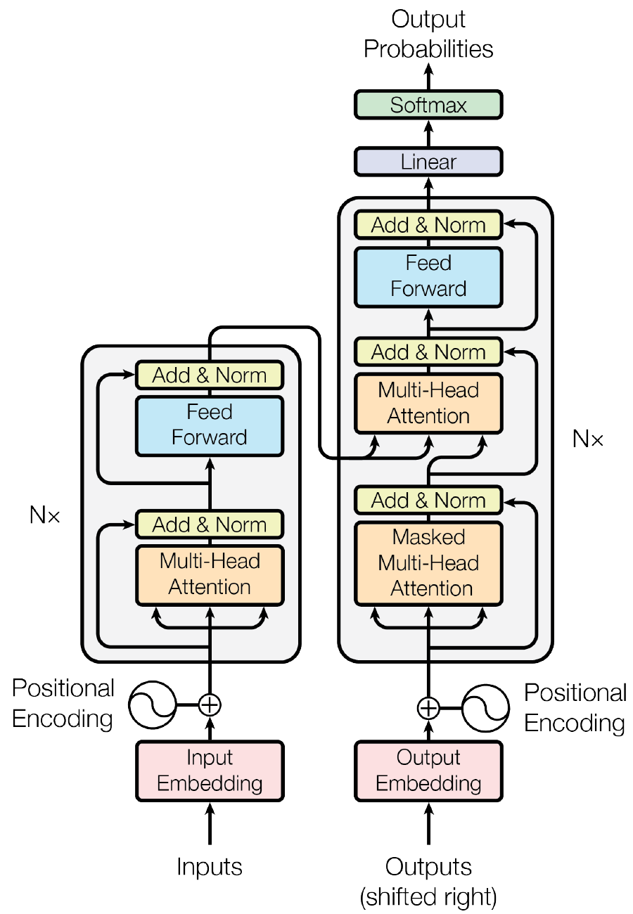
Radford et al., Section 3.1 instead use a Transformer decoder for language modeling. GPT-style decoder-only models apply causal blocks to one token sequence, without a separate encoder or encoder–decoder cross-attention.
For embedding map and positional vectors , set . To describe the computations used in caching, we consider a schematic pre-normalized block:
The feed-forward network uses , and an elementwise activation . The vocabulary map has and . Layer normalization acts on one row :
Here are learned, , and denotes coordinatewise multiplication. Normalization and the feed-forward network act tokenwise, so causal masking restricts the block's output to prefix information. This pre-normalization convention need not match every GPT.
For a fixed-length data distribution , training minimizes the expected negative log-likelihood over :
This expectation averages over data sequences, whose representations determine the attention weights. For inference, we hold the fitted parameters fixed and examine which computations generation can reuse.
3. Why a KV cache works, and why it grows
Prefill processes a prefix of tokens; decode then processes one new token at a time. At layer , the new query uses eligible prefix keys and values together with the new token's entries:
Proposition: Appending a token does not change earlier causal states
Assume fixed parameters, prefix-invariant positional encodings, no dropout, causal attention, and tokenwise normalization and feed-forward operations. Reusing the prefix's keys and values gives the same mathematical attention output as recomputing that prefix.
We argue by induction. Appending leaves earlier embeddings unchanged. If earlier states are unchanged at layer , then, for , attention uses the same positions with unchanged queries, keys and values. Therefore,
Induction establishes equality at every layer in exact arithmetic; numerical kernels can still round differently. Causality is essential because later tokens can change earlier bidirectional representations, invalidating this reuse argument.
Cache size
Let be the number of stored key/value heads, their common dimension, and bytes per scalar. Ignoring padding and metadata,
The factor two counts keys and values; the other factors count layers, positions, head coordinates, and bytes per scalar. With , , , , and two-byte scalars,
for one sequence, excluding weights and workspace. Thus caching avoids repeated prefix computation but retains linear storage growth and attention's cache-reading cost. We next examine how to reduce the width and number of stored representations.
4. Compressing the head dimension: MLA
Grouped-query attention (GQA) reduces cache width by sharing keys and values within groups of query heads; multi-query attention (MQA) uses one KV head. Multi-head latent attention (MLA) instead caches a low-dimensional representation of head-specific content keys and values.
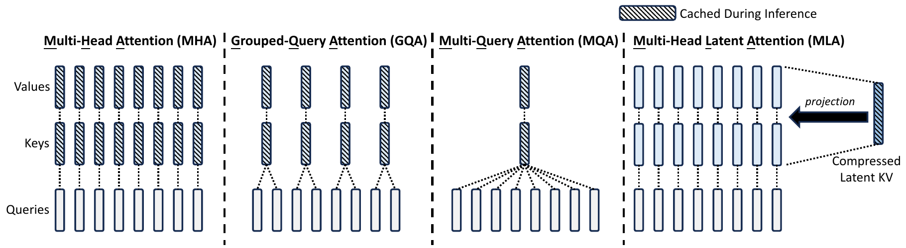
Following DeepSeek-V2, Sections 2.1.2–2.1.3, we express this low-dimensional construction in row-vector notation for head :
Here and . Associativity lets us regroup the matrix products. We apply the key projection to the query and apply the value projection after taking the weighted sum. Attention can then use cached without storing the expanded content keys and values.
Rotary position embedding (RoPE) uses position-dependent rotations to encode token positions. These rotations complicate the preceding regrouping of projections. MLA therefore keeps a separate positional key :
The cache therefore retains the pair , not only , giving equal-precision storage
MLA reduces width but retains the factor : different layers still store different latents. We next consider sharing these representations across layers.
5. Compressing the layer dimension: shared global memory
In You Only Cache Once (YOCO), Section 2, a lower causal stack produces representations for one global cache:
Each upper layer computes its own query but attends to these same cached vectors:
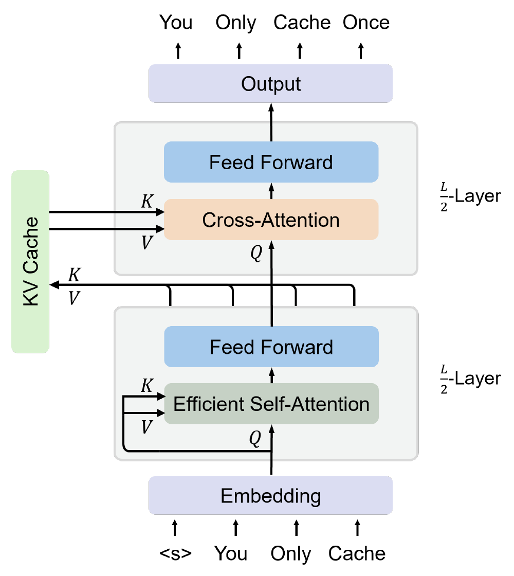
If each global cache row occupies bytes and each of layers retains at most local rows of bytes, the storage count is
rather than for layer-specific global caches. Sharing removes the global depth factor, while the second term retains bounded local states.
Shared memory does not mean shared outputs
To see why sharing need not give identical outputs, take shared scalar keys and values . For scalar query ,
The queries use identical memory but produce different attention outputs. Layer-specific output maps, residual connections, and feed-forward networks further distinguish their hidden states.
This sharing is built into the trained architecture; copying one layer's cache into arbitrary layers of an already trained decoder generally changes its function.
6. DeepSeek's causal encoder–decoder
DeepSeek-V4.1-Flash also separates an encoder from an upper decoder. Unlike the original translation encoder, its encoder is causal and cannot inspect future tokens. In Section 2.2, Equation (1), decoder global-cache projections use the final encoder states:
Here supplies global-cache entries and their compression weights. These layer-dependent projections need not produce identical caches. Compressed Sparse Attention 2 (CSA2) specifies which layers create a cache and which reuse it.
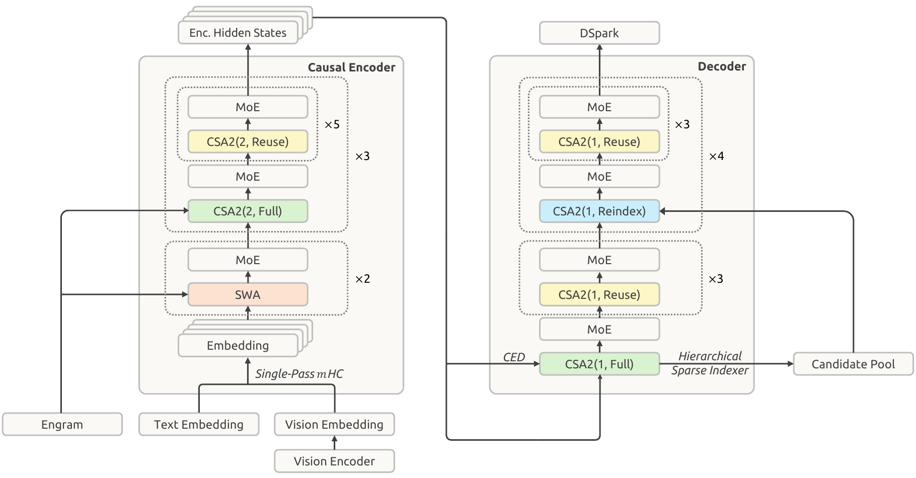
To distinguish stored caches from their readers, let identify a cache-producing layer with global state
An indexer uses keys in to select entries, which the main attention operation then reads from . Compressing nonoverlapping source blocks at ratio gives roughly rows; leaves the sequence length unchanged. At any position, the model can select only entries constructed from tokens available by that point.
Alongside global memory, each layer retains sliding-window keys and values from its own hidden states. The window length bounds this layer-specific local cache independently of .
7. Full, Reindex, and Reuse
To distinguish cache reuse from selection, fix position . Let denote layer 's score for eligible global entry , with at most entries selected. With a fixed tie rule,
where is the causally available index set for cache . This selected support specifies positions to retain; main attention then weights them using the layer's current query.
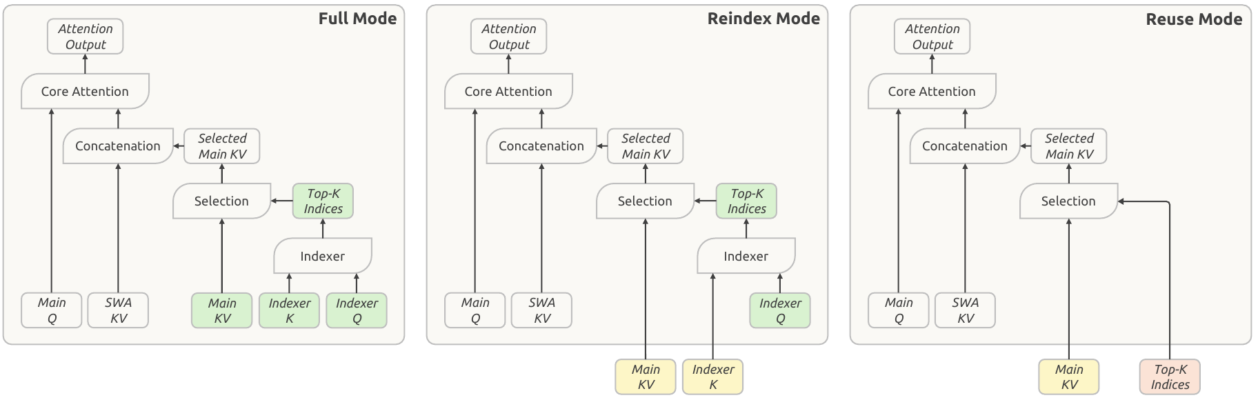
| Mode | Main KV and indexer keys | Selected positions | Main query and local KV |
|---|---|---|---|
| Full | Produce a new cache | Compute new Top-K | Compute in this layer |
| Reindex | Reuse the preceding cache | Rescore its keys and compute new Top-K | Compute in this layer |
| Reuse | Reuse the preceding cache | Reuse the latest compatible Top-K | Compute in this layer |
The modes distinguish storing entries, selecting positions, and computing attention weights. Reusing the selection does not copy the softmax weights.
For an illustrative head, let denote keys and values represented by the shared cache. At layer , attention combines selected global entries with the local window:
We write separate global and to describe the computation, although the implementation retains a shared compact representation rather than these expanded arrays.
Input: Fixed prefix, trained parameters, layer assignments to attention modes, causal entry masks, window length , and selection budget .
Output: The next-token distribution and updated caches.
- for each layer in network order do
- Compute the current queries and update this layer's local sliding-window KV.
- if the layer uses only sliding-window attention (SWA) then apply local attention and the remaining block operations; continue to the next layer.
- if mode is Full then create or update and select from eligible entries.
- else if mode is Reindex then retain , compute new indexer queries, and select a new .
- else retain and use the latest selected from this same cache.
- end if
- Recompute attention weights using the current main query, selected global entries, and current local KV; apply the remaining block operations.
- end for
- return the vocabulary softmax and updated caches.
The pseudocode summarizes cache reuse, not the complete distributed inference implementation. Decoder Full layers construct their cache from ; hierarchical indexing below further restricts decoder Reindex searches.
8. Counting the saved bytes
Because several layers read the same cache, we count each stored tensor once. Let contain distinct global-cache owners, with bytes per main-KV-plus-indexer row:
Here covers selection and candidate-pool workspace. With equal compression ratio and row size , sharing reduces the leading global term from approximately to . The ratio compares global-cache storage, not total GPU memory or wall-clock speed.
The paper's cache layout
In Section 4.2.1, three encoder layers produce ratio-two caches and one decoder layer produces a ratio-one cache. Counting these four caches gives, apart from incomplete blocks,
Converting rows to bytes requires counting quantized values and scales. Section 2.4.4 stores the 512-channel main latent as four-bit values with an eight-bit scale per 16 channels, giving
The 128-channel indexer key uses MXFP4 with a standard block size of 32 and an eight-bit scale. Including its storage gives
This recovers the report's global-cache count: approximately GB at one million tokens in decimal units, excluding local states, allocation padding, weights, and temporary workspace. Its approximately fourfold reduction relative to V4-Flash combines architectural and precision changes, not cross-layer sharing alone.
9. Avoiding repeated searches over the whole context
Although Reindex layers share keys, each could still score all available entries. The hierarchical sparse indexer reduces repeated searches by selecting a candidate pool for later indexers.
We partition positions into blocks of size at most . From the first decoder Full layer's scores , we select blocks by their maximum scores, then entries within their union:
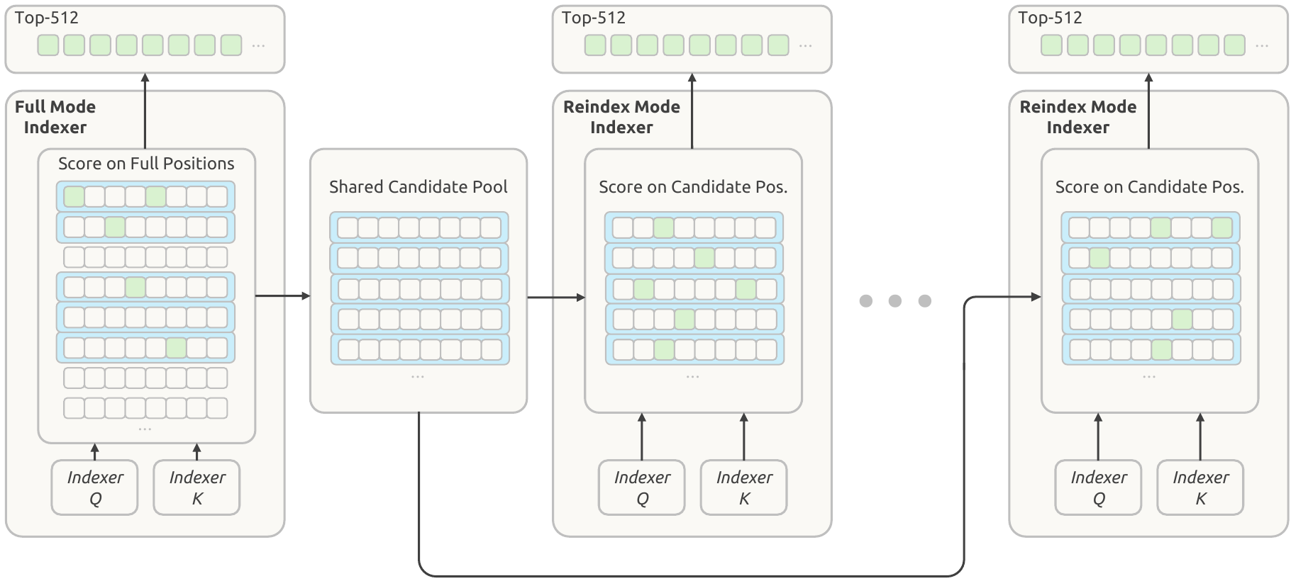
With later indexers and fixed score-evaluation cost, the number of positions scored decreases from
The first pass still depends on context length. With the paper's , , and , later queries select subsets from at most positions rather than the entire million-token history. This score-evaluation count excludes Top-K selection, attention, projections, and other block operations.
What is lost by restricting the support?
Restricting the pool can exclude useful entries. To bound one attention output's error, fix the query, keys, and values. Let be full-attention weights, , and a nonempty retained set. Suppose and define omitted mass
Since the retained scores are unchanged, their softmax weights renormalize to give
For , let average the omitted values. We split the output into retained and omitted contributions and apply the triangle inequality:
For , the outputs agree. This bound concerns one attention output, not the complete model, and is not a theorem from the DeepSeek report. The indexer's scores can differ from the main attention scores. Its selected pool therefore need not retain most of the main attention weight, so need not be small.
10. Prefill savings and approximate local replay
Prefill also benefits from computing global decoder memory directly from , without processing every prompt position through the decoder. However, local decoder KV still requires decoder states. For prompt length and window , the report reconstructs these through bounded replay over the last prompt tokens.
We measure processed positions through layer-token evaluations at fixed width:
The encoder processes the full prompt, whereas the decoder processes the replay segment. This count excludes projection and serving overheads; it does not establish half the total FLOPs for an arbitrary dense-attention Transformer.
A short window is not an exact deep receptive field
Although each layer uses a bounded window, dependencies extend across layers. For example, two layers with a two-position window and uniform scalar attention give
Because the output depends on , replaying only cannot always recover it. In Section 3.2.2, bounded replay instead approximates local states by restricting attention to
where is the replay start. During replay, prefix tokens read the cached global entries without overwriting them and rebuild approximate local states. The report acknowledges this approximation and evaluates it empirically. The earlier proof that an exact causal cache remains valid does not show that these reconstructed local states are exact.
11. Which problem does sharing solve?
We can now separate the reductions by the terms they change:
Cross-layer sharing separates cached representations from the queries used to read them, reducing storage without forcing identical outputs. Sparse selection, quantization, and bounded replay introduce separate approximations; their quality effects do not follow from the storage calculation.
This note concerns how the token policy is computed; the PPO/DPO and GRPO notes concern its training. A smaller context cache does not itself define a new policy-gradient estimator or make model parameters fit on a small device.
References
- Vaswani et al. (2017). Attention Is All You Need. Sections 3.1–3.2; Figures 1–2.
- Radford et al. (2018). Improving Language Understanding by Generative Pre-Training. Section 3.1 supplies the decoder language-model construction, not a specification of every later GPT.
- DeepSeek-AI (2024). DeepSeek-V2: A Strong, Economical, and Efficient Mixture-of-Experts Language Model. Sections 2.1.2–2.1.3; Figure 3.
- Sun et al. (2024). You Only Cache Once: Decoder-Decoder Architectures for Language Models. Sections 2.1–2.3; Figure 2.
- DeepSeek-AI (2026). DeepSeek-V4.1-Flash: Pushing the Limits of KV Cache Compression. Version 1: Sections 2.2–2.4.4, 3.2.2, and 4.2.1; Figures 3–5. The released configuration also identifies the cache-source layers, widths, and sparse-selection budgets.
- Open Compute Project (2023). Microscaling Formats (MX) Specification, version 1.0. Table 1 specifies MXFP4 element, scale, and block sizes.
The cache-invariance proof, illustrative arithmetic and readout examples, and truncation bound are worked explanations, not new model evaluations. Source figures retain their original artwork and attribution.