


Policy Gradients in Reinforcement Learning derived policy updates from sampled rewards. Language-model feedback often compares two responses instead of assigning a reward. We study two ways to learn from these comparisons: fit a reward model and optimize the policy with proximal policy optimization (PPO), or fit the policy directly with direct preference optimization (DPO).
The two approaches are connected by a reward objective that penalizes departure from a reference model using Kullback–Leibler (KL) divergence. We derive its optimal policy, use that policy to rewrite preference probabilities, and distinguish this population relationship from what either training procedure estimates.
Recap: Differentiating an expected reward
For a fixed prompt and reward that does not depend on the policy parameters, the score-function identity gives
The expectation changes with the policy. Section 4 applies this calculation to a reward with a parameter-dependent KL penalty, whose derivative must also be included. The finite-support assumptions below justify differentiation.
1. Prompts, responses, and three different policies
To keep the derivations finite, let be a finite prompt set and a finite set of valid responses to prompt . A finite vocabulary and maximum generation length suffice. A response includes its end-of-sequence token, with stopping forced by the horizon, and is padded after termination; padding is deterministic and contributes log-probability zero. We use undiscounted finite-episode returns.
For , an autoregressive language-model policy factors as
The prefix is the state, the next token is the action, and appending the token determines the next state. This is the finite-horizon interpretation from RL Foundations. Assume positive probabilities on the common valid-response support and differentiability in .
Keep three policies distinct:
| Symbol | Role | What stays fixed during an update? |
|---|---|---|
| Reference language model, often obtained by supervised fine-tuning (SFT) | Frozen throughout the alignment phase considered here | |
| Policy that generated PPO's current rollout batch | Frozen while that batch is reused | |
| Policy being optimized | Its parameters change |
The reference and rollout policies may coincide initially but need not coincide later. All logarithms are natural; all response log-probabilities below are sums over generated tokens, not length averages.
The preference-data distribution
Fix an arbitrary ordering of . A canonical pair has , so its orientation is recorded before its preference label. Define the population sampling law
Here means is preferred to . The preferred and rejected responses are when , and otherwise. Together, the prompt, pair, and label draws define the comparison distribution .
The pair distribution describes how the data were collected, including their fixed ordering. It need not sample from the current policy. For example, the pairs may have been collected earlier from an SFT model.
For the empirical analysis, assume independent comparisons . Write for their realized, oriented form. An empirical average is over these fixed records, not newly sampled model responses. Repeated judgments or dependent annotators require a different sampling analysis.
2. From comparisons to a reward model
The Bradley–Terry model assumes a finite latent score such that
This is a modeling assumption about comparisons, not a consequence of language-model pretraining. We use unit logistic scale; any alternative preference-noise scale must be included explicitly or absorbed into .
For a fitted reward model , the conditional Bernoulli negative log-likelihood becomes
where . The equality follows by orienting each pair according to its label. Adding any prompt-only constant to leaves every comparison probability unchanged.
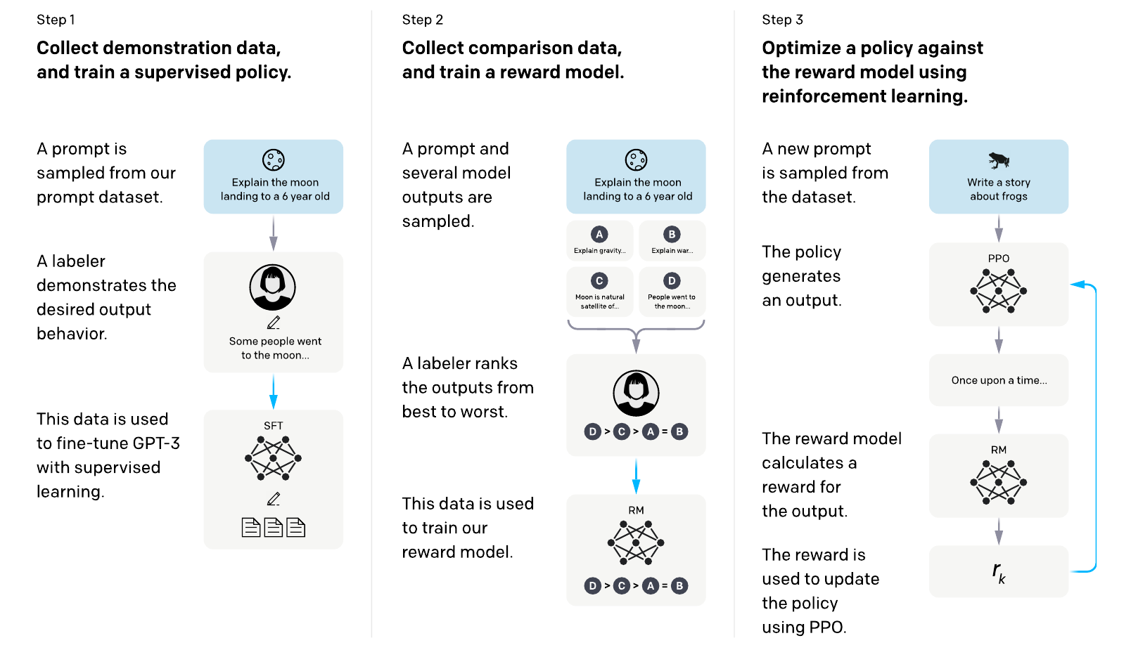
In reinforcement learning from human feedback (RLHF), this reward model can then score newly generated responses. Ouyang et al. (2022), Section 3.5 describe this SFT–reward-model–PPO pipeline. Their PPO-ptx variant also includes a pretraining-data term; the derivation here isolates the reward-minus-KL objective without that extra term.
3. Solve the KL-regularized reward problem
For now fix a reward function , reference , coefficient , and target prompt distribution . Define
Here the inner expectation draws a response from the candidate policy, while the outer expectation draws a prompt from . Neither distribution is automatically . In PPO-based RLHF, is typically a reward model fitted before the policy update. For the population connection to DPO, we will instead use the latent .
An exact optimizer and an exact objective gap
For each prompt define the partition function and exponentially tilted reference:
Finiteness of and ensures . Normalization makes a positive probability distribution. Taking logarithms gives
Next substitute this identity into the prompt-specific objective . For any response distribution , with ,
Nonnegativity of KL divergence establishes the optimizer and its gap:
Equality requires on prompts with positive probability. This is an unrestricted-policy result; a neural policy class may not contain . The reward–policy transformation is developed in Rafailov et al. (2023), Section 4 and Appendix A.1.
What the reference does
For two responses , the optimizer satisfies
The reward changes the reference odds rather than replacing them. For fixed , as ; as , mass concentrates on the reward maximizers, preserving their relative reference weights. A zero reference probability would exclude a response from any policy with finite forward KL. Positivity avoids that support obstruction in our derivations.
4. PPO: optimize the reward using rollouts
Evaluating the closed-form optimizer requires the sum over responses in , whereas PPO updates a parameterized model from sampled responses. To connect that update to the objective, we first differentiate the regularized expected reward, then introduce the clipped surrogate.
The sequence-level score identity
Let denote the joint rollout law
Hold fixed while differentiating. Write
Differentiating both the sampling probabilities and the log penalty gives
The second line uses normalization, exactly as in the policy-gradient derivation:
Thus both the extra term and any prompt-only baseline disappear after expectation. Discrete token sampling does not make the expected objective nondifferentiable; the score identity differentiates its probabilities without differentiating through a sampled token.
Why the KL cost can be assigned to tokens
The autoregressive factorization yields
Let be the distribution of the prefix generated by . The tower property gives the KL chain rule
An individual sampled log-ratio can be negative; its conditional expectation is a nonnegative KL divergence. The prefix law matters: averaging token KLs over unrelated fixed prefixes is not the sequence KL above.
At rollout iteration , freeze a fitted reward , reference , and old policy . A standard reward shaping choice on a sampled sequence is
It sums to . The terminal score can equivalently be placed at the actual termination time before deterministic padding. The frozen shaped-reward policy gradient agrees with the regularized gradient at , by the zero-score calculation above; away from that policy it is a local training construction, not the same objective for every .
The clipped token update
Let be , . The formulas assume responses are sampled from this policy. Changing the sampling temperature or removing tokens from its distribution changes that assumption.
Fit a value critic from the rollouts and obtain advantages for the shaped rewards. The critic targets the old policy's expected remaining return given ; the actor–critic note explains return and GAE estimators. In the expected surrogate below, we hold the critic fixed and treat each advantage estimate as a specified function of the rollout. During the actual batch update, we hold the recorded advantage estimates fixed.
The token likelihood ratio and clipped surrogate are
In implementation, the expectation is replaced by the rollout-batch average. Condition on that batch and its fitted advantages during the actor update. The critic, data collection, and subsequent rollout refresh are separate operations. This is the clipped actor objective of Schulman et al. (2017), Section 3, applied to the token process.
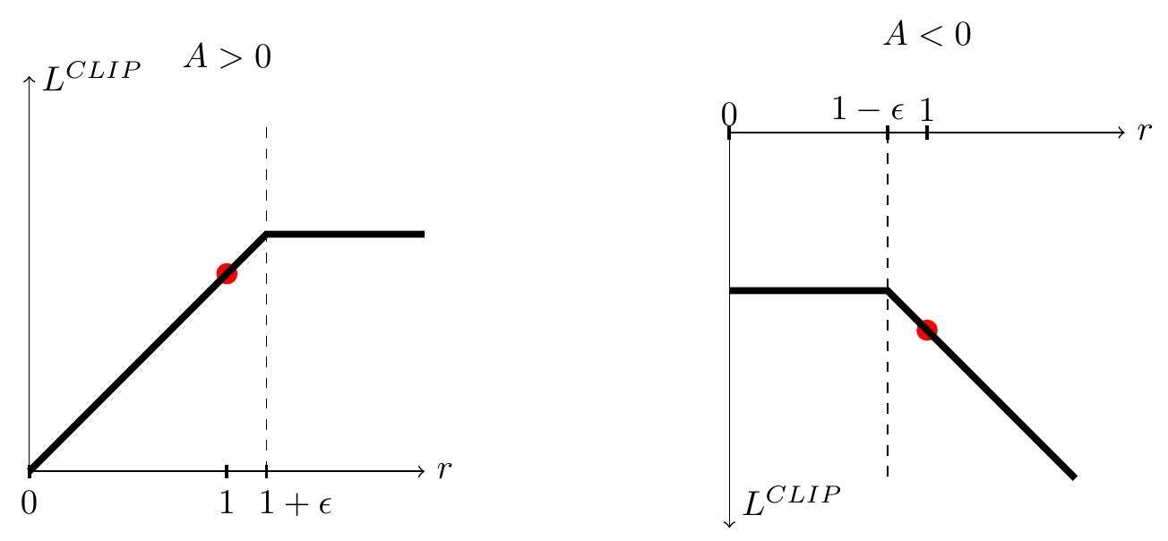
The old policy in is not the reference . Clipping discourages particular profitable ratio changes relative to ; it does not impose a hard KL bound relative to . Nor is a token ratio the whole-response ratio, which equals . These distinctions parallel the local-versus-joint clipping discussion.
5. DPO: eliminate the explicit reward model
Now use the population reward from the Bradley–Terry model and let be its unrestricted KL-regularized optimizer. The identity from Section 3 gives
Because a comparison uses the same prompt for both responses, subtracting their rewards cancels the partition term:
Consequently, the preference probability can be parameterized by a policy alone. For a candidate define the pair margin
Substitute into the conditional Bernoulli likelihood. Orienting each observed pair yields
This is the loss in Rafailov et al., equation (7) and Appendix A.2. It uses fixed preference pairs, with no newly sampled language-model rollout inside the standard DPO optimization loop. Collecting the original pairs may still have required generation and annotation.
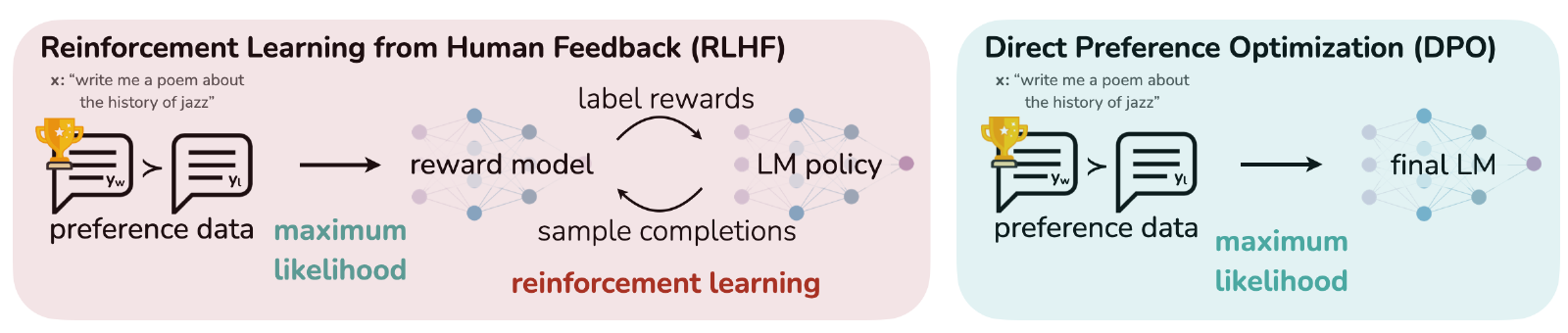
For any positive normalized candidate policy , the implicit reward
has . Its regularized optimal policy is therefore exactly . This representation is the reward-equivalence result underlying DPO; it does not say that an arbitrary learned equals the true preference reward.
The DPO gradient
For one oriented pair, set and . Since and is frozen,
Each sequence score is a token sum:
A gradient-descent update increases this pair's margin to first order by for learning rate . Poorly fitted or reversed comparisons receive more weight through . Shared parameters mean that other pairs' margins, and even a preferred response's absolute probability, need not all increase. If initially, every initial pair margin is zero and its weight is .
6. When does population DPO identify the optimal policy?
Rewriting the reward gives a preference loss, but does not yet show that fitting it determines the optimal policy. That requires enough observed comparisons to identify relative response probabilities. The following finite-response result states the needed coverage conditions.
Proposition: identification from connected comparisons
Assume the finite setup of Section 1, , positive , and Bradley–Terry preferences generated by the finite reward . Suppose:
- Every target prompt with also has .
- At each such prompt, the undirected graph with response vertices and an edge whenever is connected.
- We minimize the population DPO risk over all positive response distributions, or over a class containing , and a global minimum is attained.
Then every population minimizer equals on the target prompts. This is a population identification statement, not a finite-sample or optimization-rate guarantee.
The Bernoulli loss determines edge probabilities
First fix a prompt and a pair. Write and . Averaging only over gives
Subtract its value at the true probability:
with equality only at . Let be the prompt-pair law. Its population risk is
The policy realizes the true probability on every pair by Section 5. Consequently,
At a global minimum, the excess risk is zero. Each summand is nonnegative, so positive edge weights imply on every observed edge. Thus the loss is minimized only at the true preference probability for each compared pair. This property, called strict propriety, is also used in logistic regression.
Connectivity determines the remaining normalization
Because the sigmoid is one-to-one, matching the edge probabilities implies
on every edge. Connectivity propagates this equality along paths, so the common value is a single constant across all responses. Thus
Finally, summing over forces , hence . Prompt coverage transfers the conclusion to every target prompt. The proof requires no assumption that the collection policy equals the optimal policy, but it does require enough comparisons to identify all relative response scores.
What missing comparisons leave unidentified
If only responses and are compared while is never compared, take a uniform reference. The policies
have the same ratio and therefore the same predicted -versus- preference probability . No number of those comparisons identifies the mass assigned to . Within a disconnected comparison graph, components can retain different normalizing constants.
Finite datasets introduce a further issue: a pair may have only one observed label even though its population preference probability is strictly between zero and one. Driving that empirical loss toward zero is not the same as recovering the population probability. With a restricted neural class, model misspecification, or incomplete optimization, the proposition's premises may also fail.
7. A two-response calculation
Fix one prompt with responses and reference probabilities , . Suppose
The Bradley–Terry reward difference is . Choose the equivalent reward , . The regularized optimum is
Now recover the same policy from the population DPO loss. For , the margin and conditional risk are
The preceding Bernoulli argument minimizes this at , hence
The 75% preference probability does not mean a 75% generation probability. The latter also depends on the reference and regularization coefficient. Here it is about 69.23%.
8. The DPO training procedure
Input: fixed preference dataset , frozen reference , positive policy , , learning rates, and update budget .
Output: fitted language-model policy .
- For each record, cache the reference response log-probabilities and , or evaluate them with frozen reference parameters.
- For :
- Draw a minibatch of record indices uniformly from ; do not generate new policy responses.
- Evaluate and by teacher forcing on the recorded tokens.
- Sum generated-token log-probabilities, including EOS; mask prompt and deterministic padding tokens.
- Compute each reference-adjusted margin and the minibatch average of .
- Update , or use a specified gradient-based optimizer.
- End for.
- Return .
Conditional on and the current , let select a record independently of previous update randomness. For its loss , uniform sampling gives
Averaging independently sampled indices preserves this equality. The gradient is unbiased for the empirical objective, not automatically for ; it does not imply that optimization finds a global population minimizer. No separate learned reward network or value critic is required by this standard DPO procedure.
9. What is shared, and what is different?
| Question | PPO-based RLHF | Standard offline DPO |
|---|---|---|
| How are preferences used? | Fit an explicit reward model | Fit a policy-induced Bradley–Terry model |
| What is averaged during the actor update? | Old-policy rollout tokens with fixed advantage estimates | Recorded preferred/rejected response pairs |
| Is new generation required during training? | New rollout batches are collected as the policy changes | Not inside the fixed-dataset optimization loop |
| What is the probability ratio? | Current token policy divided by the old rollout policy | Current response likelihood divided by the frozen reference |
| How does the reference enter? | KL-based reward shaping or a specified regularized objective | Reference-adjusted pair margins |
| What does the central derivation establish? | A policy-gradient identity and a practical clipped surrogate | A reward–policy reparameterization and a preference likelihood |
PPO is a general policy optimizer; DPO is a direct preference-learning construction, not a newer PPO clipping rule. Their shared population connection assumes the same preference reward, reference, and coefficient. Fitting with one restricted class and fitting by DPO with another need not yield identical fitted policies.
For a fixed reward, controls the exact optimizer's deviation from the reference, as Section 3 shows. In a finite-sample DPO run, however, changing changes both the classification margins and the learned implicit reward. The fixed-reward formula therefore does not guarantee monotone realized KL behavior for fitted DPO policies.
Finally, Bradley–Terry assumes a scalar reward can describe the comparisons. Annotator disagreement, systematic preference cycles, distribution shift and missing response coverage can challenge that model. Neither a lower empirical DPO loss nor a larger learned PPO reward is, by itself, a guarantee of truthfulness, safety, or improved human judgments outside the evaluated setting.
Continue with GRPO: Learning from Groups of Responses, which keeps rollout-based optimization but replaces the separately fitted value critic with group-relative comparisons of sampled rewards.
References
- Rafailov, R., Sharma, A., Mitchell, E., Ermon, S., Manning, C. D., and Finn, C. (2023). Direct Preference Optimization: Your Language Model is Secretly a Reward Model. Sections 3–5 and Appendices A.1–A.6; figure excerpt uses version 1.
- Ouyang, L., et al. (2022). Training language models to follow instructions with human feedback. RLHF pipeline, Figure 2, Section 3.5 of version 1 and equation (2).
- Schulman, J., Wolski, F., Dhariwal, P., Radford, A., and Klimov, O. (2017). Proximal Policy Optimization Algorithms. Clipped surrogate and original Figure 1.