


A validation score, simulator output, or experimental measurement may require an expensive evaluation each time we change its inputs. Bayesian optimization uses the evaluations already collected to model the unknown objective and choose the next input. We derive the Gaussian-process update and expected improvement, then prove a regret bound for a separate acquisition rule, GP-UCB.
Recap: Conditioning a Gaussian model
As in Bayesian linear regression, jointly Gaussian unknowns and observations satisfy
Here are means, is cross-covariance, and is an invertible observation covariance. The conditional mean averages over uncertainty in with fixed. For a Gaussian process, the unknowns are function values; Section 2 derives the corresponding mean and variance.
1. The objective and the observation model
Let be the feasible set and the unknown objective. Throughout, larger values are better; minimize a loss by setting . After evaluations, write
Assume the maximum exists. A query is chosen using only the preceding data. In the noisy model,
with future noise independent of and past data. Thus, conditional on and the selected ,
The observed lowercase is a realization. We can assess optimization of a fixed unknown while using a working prior for inference. The regret theorem below makes the stronger assumption that was actually drawn from that prior.
An acquisition function , computed from , selects
Evaluating uses the fitted model, not a new evaluation of . This separates the expensive outer experiment from the usually cheaper inner optimization. See Frazier (2018), Sections 2–4 for the sequential-design formulation.
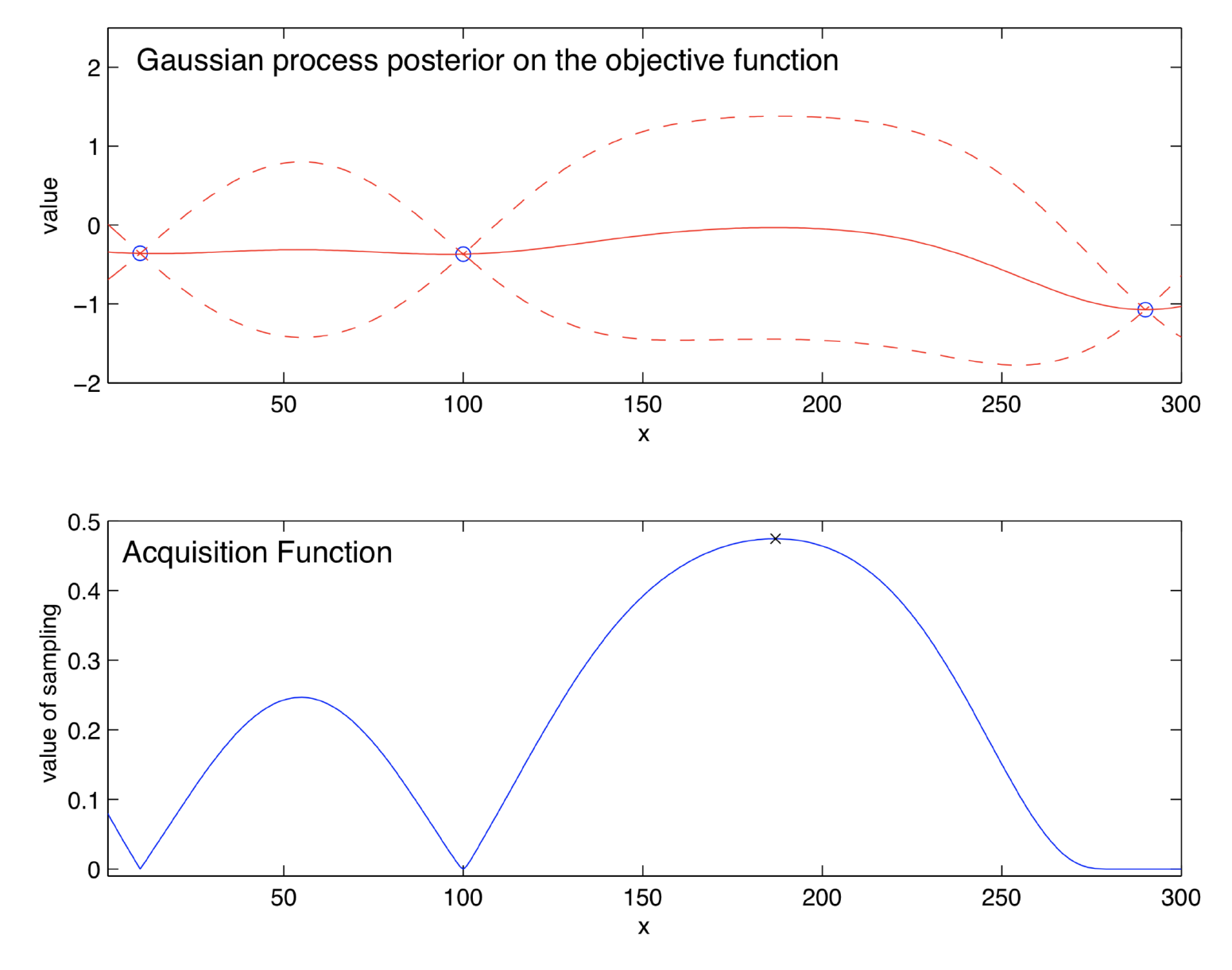
2. Deriving the Gaussian-process posterior
A Gaussian process (GP) prior is specified by a mean and a positive-semidefinite covariance kernel :
for every finite, fixed input collection , where . For example, the squared-exponential kernel is
Here is the prior marginal variance; the length scales control how quickly correlation decreases. Fix these parameters during the following derivation. As in Bayesian linear regression, conditioning updates a Gaussian prior, but here the Gaussian vector consists of function values.
Gaussian conditioning from an independent residual
First consider fixed evaluation inputs . Set
Suppose is invertible. This holds for , or for a nonsingular noiseless kernel matrix. Independent Gaussian noise gives the joint law
Define the residual
Its covariance with the observed vector vanishes:
Because is jointly Gaussian, zero covariance implies independence. Expanding the residual variance gives
Consequently, conditioning on the realized observations yields
These are the predictive equations in Rasmussen and Williams, Chapter 2, equations (2.22)–(2.24). More generally, the posterior covariance between two latent values is
Inputs are adaptive when we choose them using earlier observations. Before conditioning on that history, the observation vector need not be Gaussian. The posterior formulas still apply because each choice is determined by the recorded past data. Once we condition on that history, the choice adds no further likelihood factor involving . The sequential likelihood is proportional to . If the query rule also uses independent randomization, we can include it in the recorded history.
What the uncertainty measures
With and fixed, measures posterior uncertainty about the underlying function, not variation across new training datasets. A fresh noisy observation also includes independent measurement noise:
Use the latent standard deviation , not the noisy predictive standard deviation, in the acquisition rules derived here. When observations are noiseless and is invertible, and .
Numerically, solve linear systems. If is a Cholesky factorization, solve and . Then
A tiny diagonal jitter stabilizes this computation. It is a numerical approximation, not evidence of physical observation noise.
3. Expected improvement, derived explicitly
For this section use noiseless evaluations and at least one observed point. The incumbent is the best known function value,
If only one evaluation remained and the final recommendation had to be an evaluated point, observing would improve the incumbent by , where . Expected improvement (EI) is its posterior average:
The data, candidate , and incumbent stay fixed inside this expectation. Let , , and . Writing , with , gives
Here and are the standard-normal density and distribution function. The final equality uses symmetry and , so . Thus
The zero-variance case is a deterministic improvement, not automatically zero. At an already evaluated noiseless point it is zero because .
Holding the incumbent fixed, differentiation also makes the tradeoff precise:
For example, and cancel the extra terms when differentiating with respect to . EI favors a larger predicted value and greater uncertainty. This is a one-evaluation decision calculation; repeatedly applying it is not a proof of optimal allocation over an arbitrary remaining budget. The noiseless decision argument is developed in Frazier, Section 4.1.
With noisy observations, is not the best known latent value. Simply substituting it into this formula does not produce a noise-aware decision-theoretic EI rule. One must specify the terminal recommendation and account for uncertainty in its value; see Frazier, Section 5.1.
4. GP-UCB and a finite-domain regret guarantee
EI quantifies improvement over an incumbent. Gaussian-process upper confidence bound (GP-UCB) instead evaluates an optimistic prediction:
The exploration schedule determines how much uncertainty to include. Unlike a fixed pointwise 95% posterior interval, the schedule below controls all inputs and all rounds simultaneously. All logarithms below are natural.
Assumptions and the information quantity
Specialize to a finite nonempty set with points. Assume:
- with a known, fixed kernel satisfying .
- , , independently of ; the posterior uses this known noise variance.
- Queries depend only on previous observations; GP-UCB maximization is exact, with a fixed tie-breaking rule. Before any data, and .
The probability law below averages over both the prior draw of and observation noise. It is not a uniform guarantee for every fixed function.
For a fixed design , including repeated locations, define
Why information? For this fixed design let and independently, and put . The Gaussian entropy formula gives
The observation covariance is invertible even when the covariance of the underlying function values is singular. Below, we evaluate the log-determinant expression at the query locations selected by the algorithm. This use of the expression does not require a Gaussian law conditional only on those adaptive locations; the Gaussian calculation above assumes fixed locations.
Theorem: cumulative regret of GP-UCB
Let and
Under the assumptions above,
This is the finite-decision-set GP-prior result of Srinivas et al. (2010), Theorem 1 and Appendix A.1, with the information maximum written over query sequences so repeats are explicit.
Uniform posterior control
First fix and , and condition on . If ,
For and , symmetry and a shifted normal integral give
The failure probability for a particular is therefore at most . This bound also holds unconditionally by the tower property. If the variance is zero, conditionally almost surely, so no failure occurs. A union bound over the finite input set and all positive integers yields
Call the complementary event . It holds simultaneously at the random optimizer and the adaptively selected because it holds at every input.
Optimism bounds one-round regret
On , the UCB at is at least . Since maximizes UCB,
Also . Subtracting gives
The one-round regret is therefore bounded by uncertainty at the selected input. To control cumulative regret, we next bound the sum of these posterior uncertainties.
Posterior variances and the log determinant
For any realized query sequence, set . The Schur-complement determinant identity, a block-matrix calculation related to the identities in Linear Algebra Essentials, gives
Dividing by and iterating from the empty design establishes the pathwise identity
No independence of the selected inputs is used in this matrix identity. Moreover, . Concavity of places it above the chord between 0 and 1:
Consequently,
Finally, Cauchy–Schwarz and the nondecreasing schedule imply, on the same event ,
This proves the stated bound for every simultaneously. The UCB comparison bounds regret by posterior standard deviations, while the log-determinant identity controls their accumulated squares.
Why the bound implies learning on a fixed finite domain
A direct bound makes the asymptotic conclusion explicit. Since has rank at most , write its nonzero eigenvalues as , padding with zeros to terms. They satisfy and . Jensen's inequality for the concave logarithm gives, for every length- design ,
Maximizing over preserves the bound:
For fixed , therefore,
Also : at least one queried point has small latent regret. Identifying that point from noisy requires a recommendation rule; maximizing the noisy observations is not justified by this inequality. The result does not prove the same bound for EI, a continuous domain without additional analysis, an approximate acquisition maximizer, or an empirically retuned kernel.
5. The sequential algorithm
Input: budget , initial design of size , fixed prior and noise model, acquisition rule, feasible set, and tie-breaking rule.
Output: collected observations and a final recommendation.
- Evaluate the initial design and form .
- For :
- Compute the posterior from .
- Set in the noiseless setting, or for GP-UCB.
- Choose .
- Evaluate with the stated observation model and append .
- End for.
- Return the observations; in the noiseless case recommend the best evaluated point. With noise, specify a posterior-based recommendation or independent confirmation evaluations.
The theorem above starts GP-UCB at round 1. A separately chosen initial design is a practical variation, not literally that theorem's algorithm; its initial regret must be accounted for in a corresponding guarantee.
6. A one-dimensional Python example
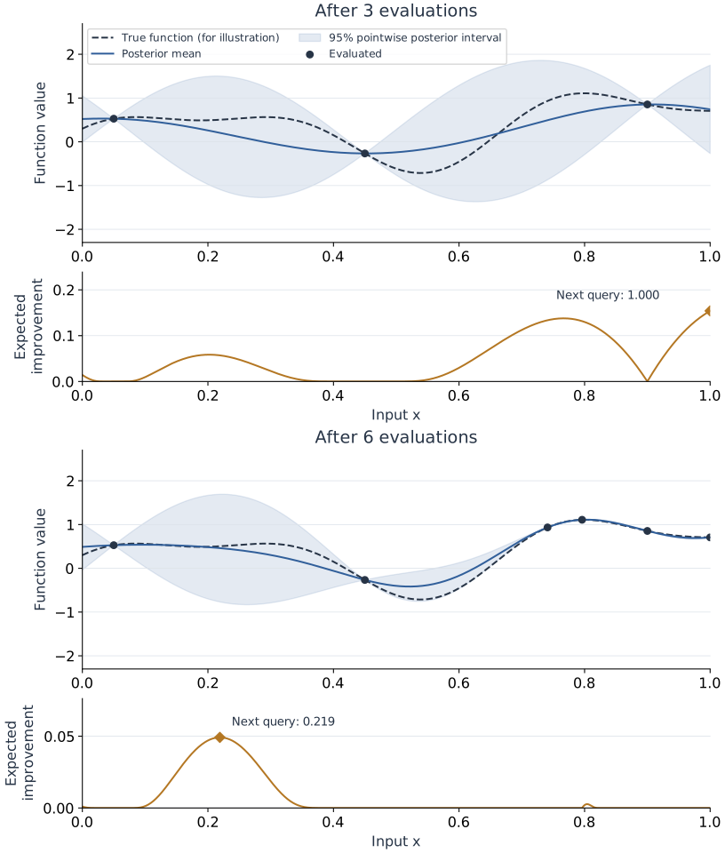
Consider the fixed, noiseless function
Use initial inputs , a zero-mean unit-variance squared-exponential GP with length scale , and EI on a 1,001-point grid. The true curve is plotted only for explanation; the selection rule receives only queried values. This illustrative fixed function is not an experiment sampled from the theorem's GP prior.
The complete Python companion implements the posterior with Cholesky solves. Its acquisition calculation includes the zero-variance limit:
import numpy as np
from scipy.special import ndtr

def expected_improvement(mu, sd, best):
    mu, sd = np.broadcast_arrays(np.asarray(mu, float),
                                 np.asarray(sd, float))
    delta = mu - best
    z = np.divide(delta, sd, out=np.zeros_like(delta), where=sd > 0)
    phi = np.exp(-0.5 * z * z) / np.sqrt(2 * np.pi)
    return np.where(sd > 0, delta * ndtr(z) + sd * phi,
                    np.maximum(delta, 0.0))
Each iteration computes the model on cheap grid points, masks previously evaluated inputs, and spends exactly one new function evaluation:
grid = np.linspace(0, 1, 1001)[:, None]
x = np.array([[0.05], [0.45], [0.90]])
y = objective(x[:, 0])
for _ in range(6):
    mu, sd = posterior(x, y, grid)
    ei = expected_improvement(mu, sd, y.max())
    available = np.min(np.abs(grid - x[:, 0]), axis=1) > 1e-8
    index = np.argmax(np.where(available, ei, -np.inf))
    x = np.vstack([x, grid[index]])
    y = np.append(y, objective(grid[index, 0]))
Here objective and posterior are defined in the companion. The jitter is numerical regularization; no measurement noise is simulated. Maximizing EI over a grid is an approximation to continuous-domain acquisition optimization.
7. Hyperparameter tuning with a fixed budget
For an RBF support-vector classifier, let encode
where is the classifier's RBF kernel parameter, called gamma by scikit-learn. It is unrelated to the information quantity . Let be fixed validation folds within the training partition, and let fit the scaling pipeline and classifier using the other folds. The expensive objective is
where and are features and labels. Conditional on the generated dataset and these folds, this objective is deterministic. The remaining search randomness comes from the seeded candidate pool and random-search ordering, not independent Gaussian observation noise.
The companion generates 500 noisy two-moons observations, reserves 25% as a test set, and compares EI with uniform random search over the same 800-point candidate pool. Before search, pool points are generated independently of the dataset. Random search follows an independent uniform permutation of the pool indices, without replacement; EI chooses among the remaining pool points. Both use the same five initial configurations and a budget of 20 objective evaluations, including initialization. Each objective evaluation comprises three classifier fits. Scaling is fitted inside each fold, preventing preprocessing leakage.
For EI, we center and scale the observed cross-validation (CV) scores at each round. The working GP uses a fixed length scale on the normalized inputs. These choices and the nonsmooth accuracy objective differ from the GP-UCB theorem's assumptions.
Snoek, Larochelle and Adams (2012) study hyperparameter optimization with GP models of the objective. We compare with random search because it is itself an effective tuning method in relevant settings (Bergstra and Bengio, 2012).
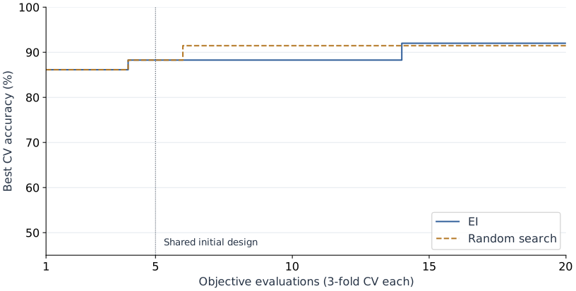
Each optimizer chooses its final configuration by CV score, refits on the full training partition, and evaluates it once on the untouched test partition. The test results are descriptive checks of the selected models, not criteria for choosing the optimizer or changing its settings. A single seed cannot establish that either method is generally better. Repeated independent runs with matched budgets would be needed for that comparison.
| Search rule | Objective evaluations | Best CV accuracy | Final test accuracy |
|---|---|---|---|
| EI | 20 | 92.00% | 96.80% |
| Random search | 20 | 91.47% | 95.20% |
These are the saved run's values, with package versions and seeds in the JSON record. Test accuracy is based on 125 held-out observations; no repeated-sample uncertainty interval is reported for this one-run illustration.
Run both examples and the numerical checks locally:
python -m pip install numpy scipy matplotlib scikit-learn
python bayesian_optimization.py --output-dir bo-output
The companion checks EI against numerical integration, its zero-variance limit, GP posterior moments against direct solves, and the variance/log-determinant identity. It exports both vector figures and a JSON record. Use --check-only to run just these mathematical checks. Download the companion first; the commands do not require a running website or external dataset.
8. What can fail in practice
- Kernel misspecification. Posterior uncertainty reflects the assumed kernel and noise model. A narrow interval is not evidence that the true function obeys them. Estimating kernel parameters adds uncertainty that plug-in predictions omit.
- Large dimension or large budgets. Acquisition search becomes harder in large spaces; an exact GP factorization costs time and storage at round . Sparse or structured alternatives change that calculation.
- Noisy incumbents. The largest noisy outcome can be a lucky measurement. Use an acquisition and recommendation rule designed for the actual observation model.
- Numerical and optimization error. Cholesky solves, input scaling and carefully chosen jitter help conditioning. Finite candidate searches or local acquisition maxima do not automatically satisfy an exact-maximization theorem.
- Constraints and costs. If feasibility is unknown or evaluations have different costs, improving alone is not the entire decision problem.
- Adaptive validation overfitting. BO repeatedly uses the same validation evidence. Keep a test set untouched until final selection and account for the full evaluation budget.
The central distinction is between modeling the objective and choosing an experiment. GP conditioning addresses the first; an acquisition rule addresses the second. The regret proof connects them only under its stated assumptions.
References
- Frazier, P. I. (2018). A Tutorial on Bayesian Optimization. Sections 3–5: GP models, acquisition functions and noisy observations.
- Rasmussen, C. E., and Williams, C. K. I. (2006). Gaussian Processes for Machine Learning, Chapter 2. Gaussian conditioning and stable posterior computation.
- Srinivas, N., Krause, A., Kakade, S. M., and Seeger, M. (2010). Gaussian Process Optimization in the Bandit Setting: No Regret and Experimental Design. Theorem 1 and Appendix A.1.
- Snoek, J., Larochelle, H., and Adams, R. P. (2012). Practical Bayesian Optimization of Machine Learning Algorithms. GP-based hyperparameter optimization.
- Bergstra, J., and Bengio, Y. (2012). Random Search for Hyper-Parameter Optimization. Random-search methodology and comparisons.