Convex Optimization: Part 1

Convex optimization is a method that finds the optimal solution by modeling a problem as a smooth landscape where every step in the right direction leads closer to the best answer. Imagine a crawler robot tasked with reaching the summit of a gently curved, dome-shaped mountain: because the terrain continuously slopes upward without any hidden dips or traps, the robot can reliably follow the gradient of the slope, taking small steps that always bring it higher until it reaches the top. Similarly, in convex optimization, the problem is shaped so that if you make a local improvement, you’re assured that you are moving toward the overall best solution. Another intuitive example is tuning a machine for peak performance, by making gradual, systematic adjustments and measuring improvement, you can confidently zero in on the setting that maximizes efficiency.

Convex optimization is a versatile tool used across countless fields, ranging from engineering and computer science to economics and biology, among others. Whether it’s fine-tuning financial portfolios, optimizing power distribution in smart grids, enhancing image quality in digital cameras, or calibrating control systems in robotics, convex optimization provides the reliable, step-by-step framework that ensures the best possible outcome.

In this blog series, we'll explore:

• How to determine if a function is convex.
• Properties and operations that preserve convexity.
• Standard forms of convex optimization problems.
• The Karush-Kuhn-Tucker (KKT) conditions: what they are and when they apply.
• Mathematical derivations, with an SVM-like example and various convex loss functions.
• A broad survey of commonly used convex functions in optimization.

Series Division:

• Part 1: Fundamentals, Convexity Criteria, and Examples.
• Part 2: Duality, KKT Conditions, and Advanced Applications.
• Part 3: Convex Loss Functions.

1. Identifying Convex Functions

A function $f: \mathbb{R}^n \to \mathbb{R}$ is convex if and only if, for all $x, y \in \mathbb{R}^n$ and all $\theta \in [0,1]$,

$$f(\theta x + (1-\theta) y) \;\le\; \theta f(x) + (1-\theta)\,f(y).$$

1.1 First-Order and Second-Order Criteria

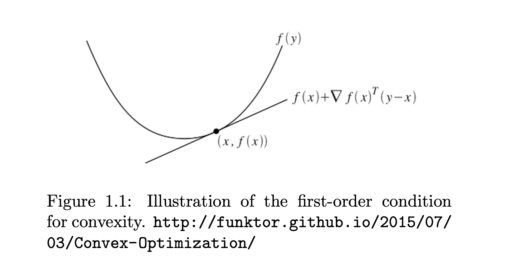
1. First-Order Test (if $f$ is differentiable):

   $$f(y) \;\ge\; f(x) \;+\; \nabla f(x)^\top (\,y - x\,), \quad \forall\,x, y.$$

   This means the function always lies above all its linear (first-order) approximations. We can draw a tangent line at any fixed point x such that $f(y) \;=\; f(x) \;+\; \nabla f(x)^\top (\,y - x\,)$. The tangent line always lies below the convex function $f(y) \;\ge\; f(x) \;+\; \nabla f(x)^\top (\,y - x\,)$.

2. Second-Order Test (if $f$ is twice differentiable):

   $$\nabla^2 f(x) \;\succeq\; 0, \quad \forall\, x.$$

   i.e. the Hessian is positive semidefinite at every point $x$.

A matrix (typically symmetric) is positive semidefinite (PSD) if for every vector $z$ the quadratic form $z^T A z$ is greater than or equal to zero.

How to check:

• Eigenvalue Method: Compute the eigenvalues of $A$. If all eigenvalues are nonnegative, $A$ is PSD.
• Principal Minors: For small matrices, you can also check that all principal minors (determinants of the top-left submatrices) are nonnegative.

This means that no matter which direction you “test” the matrix with a vector, the resulting value will not be negative.

Below are some important examples demonstrating these criteria in action—some are convex, one is not.

1.2 Preserving Convexity

Convex functions are preserved under certain operations. Here are some key closure properties:

• Nonnegative Weighted Sum: If $f_i$ are convex and $\alpha_i \ge 0$, then $\sum_{i}\alpha_i f_i$ is convex.

• Affine Transformation: If $f$ is convex, then $g(x) = f(Ax + b)$ is convex for any matrix $A$ and vector $b$.

• Pointwise Maximum: If $f_i$ are convex, then $\max_i f_i(x)$ is convex.

• Composition with a Nondecreasing Convex Function: If $f$ is convex and nondecreasing in each argument, and $g$ is convex with nonnegative components, then $x \mapsto f(g(x))$ is convex.

---

2. Examples

2.1 Quadratic Function

Consider the univariate quadratic

$$f(x) = ax^2 + bx + c,\quad a\ge 0,$$

or the multivariate version

$$f(x) = x^\top A\,x \;+\; b^\top x \;+\; c,$$

where $A \succeq 0$ (positive semidefinite).

Step-by-step check:

• Gradient (multivariate): $$\nabla f(x) = 2A\,x + b.$$
• Hessian (multivariate): $$\nabla^2 f(x) = 2A.$$
• Because $A \succeq 0,$ we have $2A \succeq 0.$ Hence, $\nabla^2 f(x)$ is positive semidefinite for all $x,$ implying convexity.

Interpretation: Quadratics with a PSD coefficient matrix are "bowl-shaped," never curving downward.

---

2.2 Log-Sum-Exp

Define

$$f(x) = \log\!\Bigl(\sum_{i=1}^n e^{x_i}\Bigr), \quad x = (x_1,\dots,x_n)\in \mathbb{R}^n.$$

Step-by-step check (Hessian test):

1. Gradient of $f(x)$:
   If we let $z = \sum_{i=1}^n e^{x_i}$, then

   $$\frac{\partial f}{\partial x_j} = \frac{1}{z} \, e^{x_j}.$$

   So the gradient is

   $$\nabla f(x) = \frac{1}{z}\,\bigl(e^{x_1}, e^{x_2}, \dots, e^{x_n}\bigr).$$

2. Hessian of $f(x)$:
   For $j,k=1,\dots,n$,

   $$\frac{\partial^2 f}{\partial x_j \partial x_k} = \frac{\partial}{\partial x_k} \Bigl(\tfrac{ e^{x_j} }{ \sum_{\ell=1}^n e^{x_\ell} }\Bigr) = \frac{e^{x_j} e^{x_k}}{z^2} \,\bigl(-\delta_{jk} + 1\bigr),$$

   where $z = \sum_{\ell=1}^n e^{x_\ell}$ and $\delta_{jk}$ is $1$ if $j=k$ and $0$ otherwise.

   More compactly, one can show

   $$\nabla^2 f(x) = \frac{1}{z}\,\mathrm{diag}(e^{x_1},\dots,e^{x_n}) \;-\; \frac{1}{z^2}\, \bigl(e^{x}\bigr)\bigl(e^{x}\bigr)^\top,$$

   which is known to be positive semidefinite. (It is a covariance-like structure because it can be viewed as the Hessian of a log-sum-exp function.)

Thus, $\nabla^2 f(x)\succeq 0$, so $f$ is convex.

Interpretation: The log-sum-exp function is a smooth approximation of $\max_i x_i$ and is widely used in machine learning (e.g., log-partition function).

---

2.3 Euclidean Norm ($p=2$)

Consider

$$f(x) = \|x\|_2 = \sqrt{x_1^2 + x_2^2 + \cdots + x_n^2},\quad x\in \mathbb{R}^n.$$

Step-by-step check (first-order or second-order approach):

1. Second-Order is trickier at $x=0$ due to non-differentiability there, so we often use a more general property: norms are always convex.

   • Geometric argument: The unit ball of $\|\cdot\|_2$ is a circle/sphere, which is convex. Hence $\|x\|_2$ is convex because it's the Minkowski functional of a convex, symmetric set.

2. Subgradient at $x\neq 0$:

   $$\nabla f(x) = \frac{x}{\|x\|_2},$$

   which does not contradict convexity (though strictly speaking, a subgradient approach is needed at $x=0$).

Thus, the Euclidean norm is convex.

General fact: $\|x\|_p$ is convex for all $p \ge 1$.

---

2.4 Non-Convex Example: $\sin(x)$

Consider $f(x) = \sin(x)$ (univariate, for simplicity).

Step-by-step check:

• First derivative: $f'(x) = \cos(x).$
• Second derivative: $f''(x) = -\sin(x).$

To be convex, we would need $f''(x) \ge 0$ for all $x$ or at least not be negative anywhere. But $-\sin(x)$ is sometimes positive, sometimes negative. In fact, for $x \in (0, \pi)$, $f''(x) = -\sin(x) < 0,$ indicating $f$ is concave in that region. Around $x=0,$ we have $f''(0)=0,$ which doesn't guarantee convexity. Overall, $\sin(x)$ is not convex over $\mathbb{R}$.

Interpretation: $\sin(x)$ oscillates, so it curves up and down infinitely often, violating any global convexity requirement.

---

Notes

1. Quadratic + PSD → Convex.
2. Log-sum-exp: Strictly convex, as it has a positive semidefinite Hessian.
3. ℓ₂-norm: Convex (more generally, ℓₚ-norms for $p \ge 1$ are convex).
4. $\sin(x)$: Not convex, since its second derivative changes sign.

General thinking process when Verifying Convexity:

• Definition Check: Confirm that for any two points $x$ and $y$ in the domain and any $\theta \in [0,1]$,

  $$f(\theta x + (1-\theta)y) \le \theta f(x) + (1-\theta)f(y).$$

  This is the fundamental property of convex functions.

• First-Order Condition: For differentiable functions, verify that the function always lies above its tangent lines. In other words, check that

  $$f(y) \ge f(x) + \nabla f(x)^T (y-x)$$

  holds for all $x$ and $y$.

• Second-Order Condition: For twice differentiable functions, check that the Hessian matrix is positive semidefinite everywhere in the domain. This guarantees that the curvature is non-negative throughout (and watch for points of non-differentiability).

• Composition Rules: Many functions are built from simpler components. Convexity is preserved under operations such as:

  • Sum: If $f(x)$ and $g(x)$ are convex, then

    $$h(x) = f(x) + g(x)$$

    is convex.

  • Scaling: If $f(x)$ is convex and $a \ge 0$ is a scalar, then

    $$g(x) = a \, f(x)$$

    is convex.

  • Affine Transformation: If $f$ is convex and $g(x) = A x + b$ is an affine mapping, then

    $$h(x) = f(A x + b)$$

    is convex.

  • Nondecreasing/Nonincreasing Composition:
    If $f:\mathbb{R}\to\mathbb{R}$ is convex and nondecreasing and $g:\mathbb{R}^n\to\mathbb{R}$ is convex, then

    $$h(x) = f(g(x))$$

    is convex.
    Similarly, if $f$ is convex and nonincreasing and $g$ is concave, then $h(x)=f(g(x))$ is convex.

  • Pointwise Maximum: The pointwise maximum of convex functions is also convex. If $f_i(x)$ are convex for $i = 1, 2, \dots, n$, then

    $$h(x) = \max\{f_1(x), f_2(x), \dots, f_n(x)\}$$

    is convex.

  • Perspective Function: Given a convex function $f:\mathbb{R}^n\to\mathbb{R}$, its perspective

    $$g(x,t) = t \, f\Bigl(\frac{x}{t}\Bigr)$$

    is convex on $\{(x,t) \in \mathbb{R}^{n+1}: t > 0\}$. This is particularly useful for scaling or normalization.

  • Elementwise Composition: When $g(x)$ applies a convex (or concave) function elementwise to a vector $x$, and $f(z)$ aggregates those values via a convex operation (like a sum or a norm), the overall function remains convex under suitable conditions. For example, if $f(z)=\|z\|_2$ is convex and $g(x)$ yields a vector of convex transformations of $x$, then $h(x)=\|g(x)\|_2$ can be convex.

• Reformulation: If the convexity of the original function is not immediately clear, try to reformulate it as a combination of simpler convex components. This can often reveal the hidden structure.

• Convex Relaxation: For non-convex functions, a common approach is to approximate them with a surrogate convex function that shares its desired properties. This method makes the problem easier to analyze and solve.

• Additional Tools: When analytical methods are challenging, numerical verification or symbolic computation tools can provide further insights into the function’s behavior.

Often, just one of these checks is enough to show a function is convex, so pick the approach that fits your problem best. Together, these strategies give you a clear and practical toolkit for tackling even the toughest optimization challenges.

This concludes Part 1 of the series on convex optimization, where I covered the fundamentals, convexity criteria, and illustrative examples. To continue your exploration of this topic, you can check out Part 2: Duality, KKT Conditions, and Advanced Applications and Part 3: Convex Loss Functions for a deeper dive into these advanced concepts.

References & Further Reading

1. Boyd, S., & Vandenberghe, L. (2004). Convex Optimization. Cambridge University Press.
2. Hastie, T., Tibshirani, R., & Friedman, J. (2009). The Elements of Statistical Learning.
3. Schölkopf, B., & Smola, A. (2001). Learning with Kernels. MIT Press.
4. García-Gonzalo, E., et al. (2016). A Study on Kernel Methods for Classification.