Bayesian Linear Regression: Fundamentals, Ridge, and Lasso Regularization

Bayesian linear regression provides a probabilistic framework for modeling the relationship between predictors and a response variable. In this framework, model parameters are treated as random variables, and we derive a full posterior distribution for them rather than just point estimates. In the sections below, we first detail the standard Bayesian linear regression model and then extend the discussion to two popular regularization methods: Bayesian Ridge and Bayesian Lasso.

Key Bayesian Regression Framework

Model Setup and Notation

We begin with the familiar linear model:

\mathbf{y} = \mathbf{X}\boldsymbol{\beta} + \boldsymbol{\epsilon},

where:

$\mathbf{y}$ is an $n \times 1$ response vector,
$\mathbf{X}$ is an $n \times (p+1)$ design matrix (including a column for the intercept),
$\boldsymbol{\beta}$ is a $(p+1) \times 1$ vector of unknown coefficients, and
the errors $\boldsymbol{\epsilon}$ are assumed to be independent and normally distributed as

\boldsymbol{\epsilon} \sim N(\mathbf{0}, \sigma^2 \mathbf{I}).

Standard Bayesian Linear Regression

Likelihood

In the Bayesian framework, we combine the data likelihood with a prior distribution on the parameters. In statistical modeling, the likelihood function represents the probability of observing the data $\mathbf{y}$ given the parameters $\boldsymbol{\beta}$ and $\sigma^2$ . For our linear model, with independent normally distributed errors, the likelihood function is given by:

L(\boldsymbol{\beta}, \sigma^2) = p(\mathbf{y} \mid \boldsymbol{\beta}, \sigma^2) = \prod_{i=1}^{n} \frac{1}{\sqrt{2\pi\sigma^2}} \exp\!\left(-\frac{(y_i - \mathbf{x}_i^T \boldsymbol{\beta})^2}{2\sigma^2}\right),

where $\mathbf{x}_i^T$ is the $i$ th row of $\mathbf{X}$ . This can be simplified as:

p(\mathbf{y} \mid \boldsymbol{\beta}, \sigma^2) \propto \exp\!\Bigl(-\frac{1}{2\sigma^2}\|\mathbf{y} - \mathbf{X}\boldsymbol{\beta}\|^2\Bigr).

Prior

In the Bayesian setting, we treat $\boldsymbol{\beta}$ as a random variable. A common (noninformative or weakly informative) choice is to assume a Gaussian prior on $\boldsymbol{\beta}$ , which is conjugate to the Gaussian likelihood. This leads to analytic solutions and simplifies computation:

\boldsymbol{\beta} \sim N\Bigl(\mathbf{0},\, \sigma^2 \tau^{-1} \mathbf{I}\Bigr),

where $\tau$ controls the spread or uncertainty of our prior relative to the noise variance $\sigma^2$ .

However, the Gaussian prior is not the only choice. Depending on the application and prior beliefs, different priors can be used:

Noninformative Prior: When little prior knowledge is available, one might use a flat or uniform prior over $\boldsymbol{\beta}$ i.e. $p(\boldsymbol{\beta}) \propto 1$ . This approach does not favor any particular values and lets the data speak for itself.
Weakly Informative Gaussian Prior: In many cases, a Gaussian prior with a large variance (small $\tau$ ) is used to provide mild regularization without imposing strong beliefs. This is particularly useful for stabilizing estimates in the presence of multicollinearity.
Laplace Prior (Double-Exponential): For scenarios where sparsity is desired, such as in variable selection, a Laplace prior can be imposed on each coefficient. This is the basis for the Bayesian Lasso:
$p(\beta_j) = \frac{\lambda}{2} \exp\!\left(-\lambda |\beta_j|\right).$
Heavy-Tailed Priors: In some applications, it might be appropriate to use heavy-tailed distributions like the Student's t-distribution as a prior for $\boldsymbol{\beta}$ . Such priors are more robust to outliers in the data and allow for occasional large coefficient values.

The choice of prior should reflect any prior knowledge or assumptions about the parameters. For example, if prior studies suggest that most predictors have a negligible effect on the response, a Laplace prior might be preferred to encourage sparsity. Conversely, if one has reason to believe that the effects are normally distributed around zero with moderate variance, a Gaussian prior is appropriate.

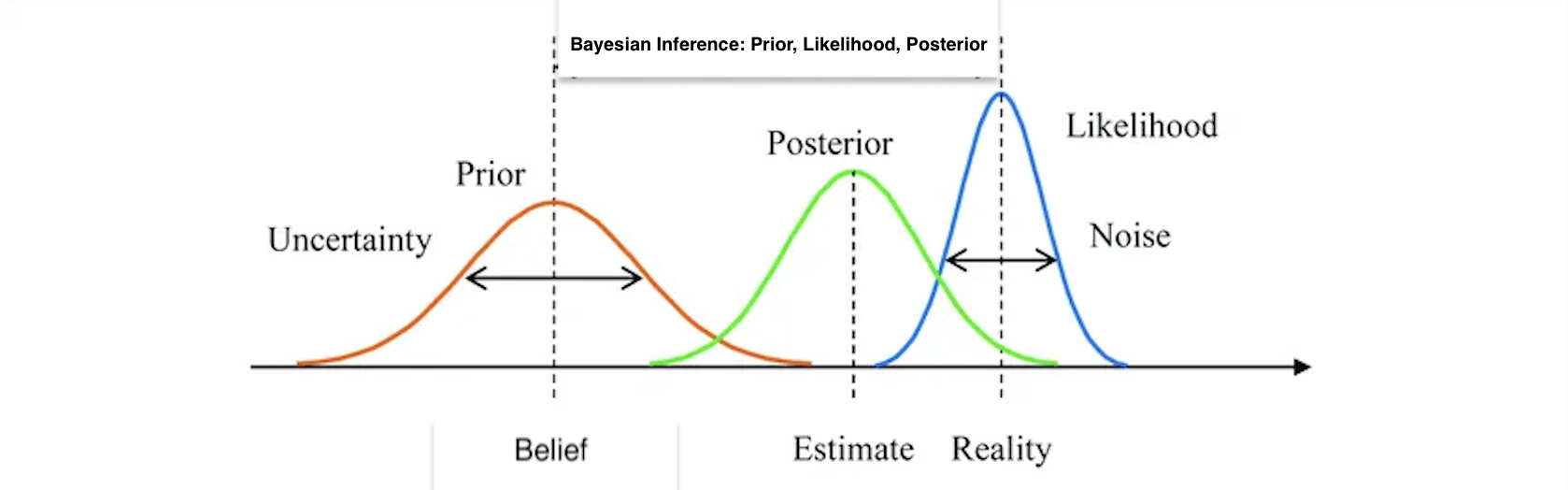
Posterior: Combine Likelihood and the Prior

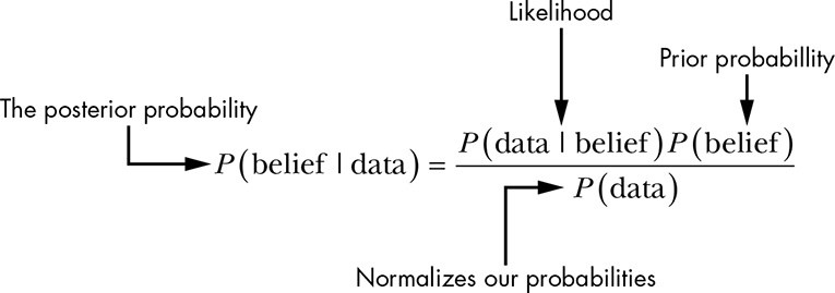
Bayesian inference uses Bayes’ rule in the form:

p(\boldsymbol{\beta} \mid \mathbf{y}) \;=\; \frac{p(\mathbf{y}, \boldsymbol{\beta})}{p(\mathbf{y})}=\; \frac{p(\mathbf{y} \mid \boldsymbol{\beta}) \;\times\; p(\boldsymbol{\beta})}{p(\mathbf{y})}.

Next, we write the marginal likelihood $p(\mathbf{y})$ by integrating over all possible $\boldsymbol{\beta}$ :

p(\mathbf{y}) \;=\; \int p(\mathbf{y}, \boldsymbol{\beta}) \,\mathrm{d}\boldsymbol{\beta} \;=\; \int p(\mathbf{y} \mid \boldsymbol{\beta}) \;\times\; p(\boldsymbol{\beta}) \,\mathrm{d}\boldsymbol{\beta}.

However, computing $p(\mathbf{y})$ (the marginal likelihood) can be challenging because it involves integrating over all possible parameter values. That is why we often write the posterior up to a proportionality constant. The posterior distribution for $\boldsymbol{\beta}$ is proportional to the product of the likelihood and the prior:

p(\boldsymbol{\beta} \mid \mathbf{y}) \;\propto\; p(\mathbf{y} \mid \boldsymbol{\beta}) \;\times\; p(\boldsymbol{\beta}).

Therefore, for our setup the posterior distribution is:

p(\boldsymbol{\beta} \mid \mathbf{y}, \sigma^2) \propto p(\mathbf{y} \mid \boldsymbol{\beta}, \sigma^2) \times p(\boldsymbol{\beta}).

Because both the likelihood and the prior are Gaussian, the posterior for $\boldsymbol{\beta}$ is also Gaussian. This conjugacy yields an analytic solution for the posterior, allowing us to quantify the uncertainty over the coefficients.

Posterior Distributions: Analytic and Approximate Forms

The posterior distribution arises when we update our beliefs about parameters after observing data, capturing both our prior assumptions and the information contained in the likelihood. In some situations—especially when the chosen prior and likelihood form a convenient pairing—the necessary integrals can simplify, leading to an exact, closed-form expression for the posterior.

In certain cases, the likelihood and prior are chosen to be conjugate. This means the resulting posterior has the same functional form as the prior, making it possible to derive a closed-form (analytic) solution easily. These so-called "conjugate" relationships are not the only way to obtain analytic solutions, but in most practical cases, the marginal likelihood integrals become too complex to solve directly.

Non-Analytic Example: Bayesian Logistic Regression

Model Setup

Likelihood

Suppose $\mathbf{y}\in \{0,1\}^n$ are binary outcomes and $X$ is the design matrix. For logistic regression, each $y_i$ is modeled with

P\bigl(y_i = 1 \mid \mathbf{x}_i,\boldsymbol{\beta}\bigr) \;=\; \sigma\!\bigl(\mathbf{x}_i^\mathsf{T}\,\boldsymbol{\beta}\bigr),

where $\sigma(z) = \tfrac{1}{1+e^{-z}}$ is the logistic function. The likelihood for all $n$ data points is:

p(\mathbf{y} \mid \boldsymbol{\beta}) \;=\; \prod_{i=1}^n \sigma\!\bigl(\mathbf{x}_i^\mathsf{T}\boldsymbol{\beta}\bigr)^{\,y_i} \Bigl(1 - \sigma\!\bigl(\mathbf{x}_i^\mathsf{T}\boldsymbol{\beta}\bigr)\Bigr)^{\,1 - y_i}.

Prior

We can again choose a Gaussian prior for $\boldsymbol{\beta}$ :

p(\boldsymbol{\beta}) \;=\; \mathcal{N}\bigl(\boldsymbol{\mu}_0,\;\Sigma_0\bigr).

Posterior Challenge

Form of the Posterior

Using Bayes’ rule, the posterior is:

p(\boldsymbol{\beta} \mid \mathbf{y}) \;\propto\; \underbrace{\prod_{i=1}^n \sigma\!\bigl(\mathbf{x}_i^\mathsf{T}\boldsymbol{\beta}\bigr)^{\,y_i} \bigl[\,1 - \sigma\!\bigl(\mathbf{x}_i^\mathsf{T}\boldsymbol{\beta}\bigr)\bigr]^{1 - y_i}}_{\text{Logistic likelihood}} \;\times\; \underbrace{\exp\!\Bigl(-\tfrac12\bigl(\boldsymbol{\beta}-\boldsymbol{\mu}_0\bigr)^\mathsf{T}\Sigma_0^{-1}\bigl(\boldsymbol{\beta}-\boldsymbol{\mu}_0\bigr)\Bigr)}_{\text{Gaussian prior}}.

The presence of the logistic function $\sigma(\cdot)$ in the product creates a non-conjugate relationship with the Gaussian prior.

No Closed-Form Integral

Unlike the Gaussian–Gaussian case, the integral

p(\mathbf{y}) \;=\; \int p(\mathbf{y},\boldsymbol{\beta})\,d\boldsymbol{\beta} \;=\; \int p(\mathbf{y} \mid \boldsymbol{\beta})\,p(\boldsymbol{\beta})\,d\boldsymbol{\beta}

does not simplify into any known closed-form solution. This makes the posterior analytically intractable.

As a result, we often rely on numerical approaches such as Markov Chain Monte Carlo (MCMC), variational inference, or other approximation methods to explore or estimate the posterior distribution. These techniques ensure that even when an exact solution is not feasible, we can still capture the uncertainty about our parameters and make informed inferences from the data.

By working with a full posterior distribution, Bayesian linear regression enables the incorporation of prior information and provides a way to capture uncertainty. Instead of a single point estimate for each $\beta_j$ , you get a distribution reflecting all plausible values and their corresponding probabilities.

Bayesian Ridge Regression

In Bayesian Ridge Regression, we use the same Gaussian prior:

\boldsymbol{\beta} \sim N\Bigl(\mathbf{0},\, \sigma^2 \tau^{-1} \mathbf{I}\Bigr).

Likelihood:
The likelihood function remains:

p(\mathbf{y} \mid \boldsymbol{\beta}, \sigma^2) \propto \exp\!\Bigl(-\frac{1}{2\sigma^2}\|\mathbf{y} - \mathbf{X}\boldsymbol{\beta}\|^2\Bigr).

Prior:
The Gaussian prior on the coefficients is:

p(\boldsymbol{\beta}) \propto \exp\!\Bigl(-\frac{\tau}{2}\boldsymbol{\beta}^T \boldsymbol{\beta}\Bigr).

Posterior:
By Bayes’ rule, the posterior is:

p(\boldsymbol{\beta} \mid \mathbf{y}, \sigma^2) \propto p(\mathbf{y} \mid \boldsymbol{\beta}, \sigma^2) \, p(\boldsymbol{\beta}) \propto \exp\!\Bigl(-\frac{1}{2\sigma^2}\|\mathbf{y} - \mathbf{X}\boldsymbol{\beta}\|^2 - \frac{\tau}{2}\boldsymbol{\beta}^T \boldsymbol{\beta}\Bigr).

Taking the negative logarithm (and ignoring constants) gives the following objective for Maximum A Posteriori (MAP) estimation:

\min_{\boldsymbol{\beta}} \; \frac{1}{2\sigma^2}\|\mathbf{y} - \mathbf{X}\boldsymbol{\beta}\|^2 + \frac{\tau}{2}\boldsymbol{\beta}^T \boldsymbol{\beta}.

Multiplying through by $2\sigma^2$ (which does not affect the minimizer) leads to:

\min_{\boldsymbol{\beta}} \; \|\mathbf{y} - \mathbf{X}\boldsymbol{\beta}\|^2 + \sigma^2 \tau \, \|\boldsymbol{\beta}\|^2.

Derivation of the MAP Estimate:
Taking the derivative with respect to $\boldsymbol{\beta}$ and setting it to zero:

-2\mathbf{X}^T(\mathbf{y} - \mathbf{X}\boldsymbol{\beta}) + 2\sigma^2 \tau \, \boldsymbol{\beta} = 0.

Rearrange to obtain:

\mathbf{X}^T\mathbf{X}\boldsymbol{\beta} + \sigma^2 \tau \, \boldsymbol{\beta} = \mathbf{X}^T\mathbf{y}.

Thus, the MAP estimate for Bayesian Ridge Regression is:

\hat{\boldsymbol{\beta}}_{\text{BayesRidge}} = \bigl(\mathbf{X}^T\mathbf{X} + \sigma^2 \tau \, \mathbf{I}\bigr)^{-1}\mathbf{X}^T\mathbf{y}.

Bayesian Lasso Regression

Bayesian Lasso introduces sparsity by using a Laplace (double-exponential) prior on the regression coefficients.

Model, Likelihood, and Prior for Bayesian Lasso

Model:
We retain the linear model:

\mathbf{y} = \mathbf{X}\boldsymbol{\beta} + \boldsymbol{\epsilon}, \quad \text{with } \boldsymbol{\epsilon} \sim N(\mathbf{0}, \sigma^2 \mathbf{I}).

Likelihood:
The likelihood function is:

p(\mathbf{y} \mid \boldsymbol{\beta}, \sigma^2) \propto \exp\!\Bigl(-\frac{1}{2\sigma^2}\|\mathbf{y} - \mathbf{X}\boldsymbol{\beta}\|^2\Bigr).

Prior:
For Bayesian Lasso, we place a Laplace prior on each coefficient $\beta_j$ :

p(\beta_j) = \frac{\lambda}{2} \exp\!\left(-\lambda |\beta_j|\right).

For the entire coefficient vector:

p(\boldsymbol{\beta}) = \prod_{j=1}^{p} \frac{\lambda}{2} \exp\!\left(-\lambda |\beta_j|\right) \propto \exp\!\Bigl(-\lambda \|\boldsymbol{\beta}\|_1\Bigr).

Posterior and MAP Estimation for Bayesian Lasso

Posterior:
Using Bayes’ rule, the posterior distribution is given by:

p(\boldsymbol{\beta} \mid \mathbf{y}, \sigma^2) \propto p(\mathbf{y} \mid \boldsymbol{\beta}, \sigma^2) \, p(\boldsymbol{\beta}) \propto \exp\!\Bigl(-\frac{1}{2\sigma^2}\|\mathbf{y} - \mathbf{X}\boldsymbol{\beta}\|^2 - \lambda \|\boldsymbol{\beta}\|_1\Bigr).

Taking the negative logarithm (ignoring constants) yields the MAP objective:

\min_{\boldsymbol{\beta}} \; \frac{1}{2\sigma^2}\|\mathbf{y} - \mathbf{X}\boldsymbol{\beta}\|^2 + \lambda \|\boldsymbol{\beta}\|_1.

Multiplying through by $2\sigma^2$ for clarity, we have:

\min_{\boldsymbol{\beta}} \; \|\mathbf{y} - \mathbf{X}\boldsymbol{\beta}\|^2 + 2\sigma^2 \lambda \, \|\boldsymbol{\beta}\|_1.

Note:
Due to the non-differentiability of the $L_1$ norm at zero, there is no closed-form solution for the Bayesian Lasso MAP estimator. In practice, numerical methods such as Gibbs sampling, variational inference, or coordinate descent adapted for the Bayesian framework are used to estimate $\boldsymbol{\beta}$ or to sample from the full posterior.

Hyperparameter Interpretation

An important aspect of Bayesian linear regression is understanding the role of the hyperparameters. The parameter $\tau$ in the Gaussian prior (used in standard Bayesian regression and Bayesian Ridge) controls the spread of the prior distribution on $\boldsymbol{\beta}$ ; a larger $\tau$ implies a tighter prior (i.e., more shrinkage), while a smaller $\tau$ allows for greater variability in the coefficient estimates. Similarly, in Bayesian Lasso, the hyperparameter $\lambda$ governs the strength of the $L_1$ penalty, where a larger $\lambda$ encourages more coefficients to be shrunk to exactly zero, thereby promoting sparsity and enhancing variable selection. Tuning these hyperparameters is critical, as they directly affect the balance between model complexity and regularization, ultimately influencing both the predictive performance and interpretability of the model.

Summary of Bayesian Linear Regression Methods

Standard Bayesian Linear Regression:
- Model: $\mathbf{y} = \mathbf{X}\boldsymbol{\beta} + \boldsymbol{\epsilon}, \quad \boldsymbol{\epsilon} \sim N(\mathbf{0}, \sigma^2 \mathbf{I}).$
- Notation:
  $\mathbf{y}$ is an $n \times 1$ response vector, $\mathbf{X}$ is an $n \times (p+1)$ design matrix, $\boldsymbol{\beta}$ is a $(p+1) \times 1$ coefficient vector.
- Prior:
  $\boldsymbol{\beta} \sim N\Bigl(\mathbf{0},\, \sigma^2 \tau^{-1} \mathbf{I}\Bigr)$ .
- Posterior:
  $p(\boldsymbol{\beta} \mid \mathbf{y}, \sigma^2) \propto \exp\!\Bigl(-\frac{1}{2\sigma^2}\|\mathbf{y} - \mathbf{X}\boldsymbol{\beta}\|^2 - \frac{\tau}{2}\boldsymbol{\beta}^T \boldsymbol{\beta}\Bigr)$ , leading to a closed-form MAP solution akin to ridge regression.
Bayesian Ridge Regression:
- Prior:
  $\boldsymbol{\beta} \sim N\Bigl(\mathbf{0},\, \sigma^2 \tau^{-1} \mathbf{I}\Bigr)$ .
- MAP Estimator: $\hat{\boldsymbol{\beta}}_{\text{BayesRidge}} = \bigl(\mathbf{X}^T\mathbf{X} + \sigma^2 \tau \, \mathbf{I}\bigr)^{-1}\mathbf{X}^T\mathbf{y}.$
- Benefits:
  Provides shrinkage of coefficients and quantifies uncertainty via the full posterior distribution.
Bayesian Lasso Regression:
- Prior:
  Laplace prior $p(\boldsymbol{\beta}) \propto \exp\!\Bigl(-\lambda \|\boldsymbol{\beta}\|_1\Bigr)$ .
- MAP Objective: $\min_{\boldsymbol{\beta}} \; \|\mathbf{y} - \mathbf{X}\boldsymbol{\beta}\|^2 + 2\sigma^2 \lambda \, \|\boldsymbol{\beta}\|_1.$
- Benefits:
  Encourages sparsity by driving some coefficients to exactly zero, aiding in variable selection. No closed-form solution exists; numerical methods are employed.

Practical Considerations

In practice, Bayesian linear regression models are often implemented using computational techniques such as Markov Chain Monte Carlo (MCMC) methods, including Gibbs sampling or the Metropolis-Hastings algorithm, to sample from the posterior distribution. Software packages such as Stan, JAGS, or PyMC3 provide powerful tools for performing these computations, enabling the estimation of complex Bayesian models. However, practitioners should be aware of the computational challenges associated with MCMC, such as convergence diagnostics and potential slow mixing in high-dimensional parameter spaces. Variational inference is another alternative that approximates the posterior more quickly, although sometimes at the cost of reduced accuracy. These practical considerations are crucial when applying Bayesian methods to real-world datasets.

Bayesian linear regression not only yields point estimates for the coefficients but also provides a full probabilistic description of uncertainty. By incorporating regularization through Bayesian Ridge and Bayesian Lasso, we obtain models that are robust to overfitting and multicollinearity, while also offering valuable insights through the posterior distributions.