
Convex Optimization: Part 3
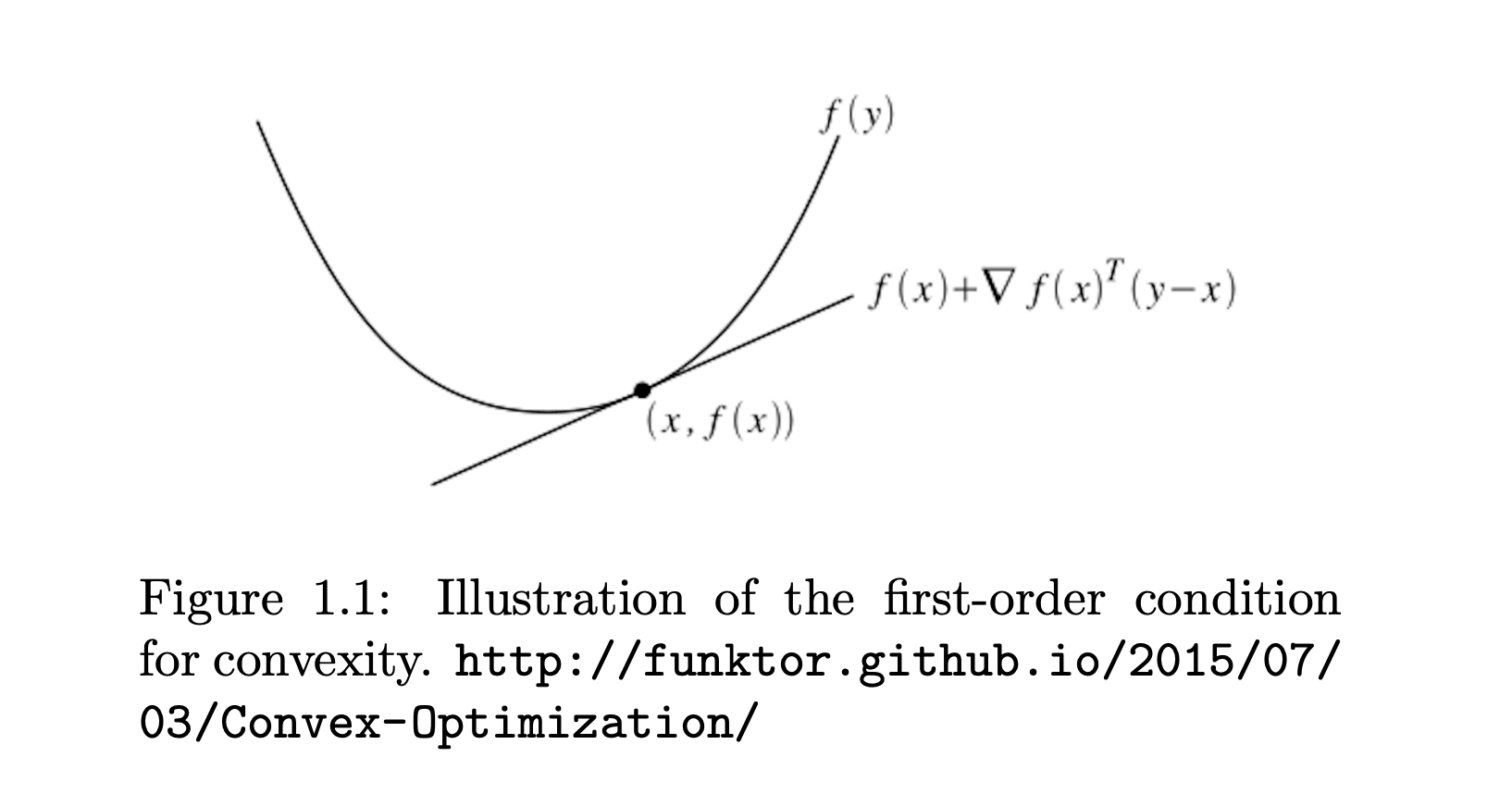
Image credit: Huang et al. (2022)
In this blog series, we are exploring:
- How to determine if a function is convex.
- Properties and operations that preserve convexity.
- Standard forms of convex optimization problems.
- The Karush-Kuhn-Tucker (KKT) conditions: what they are and when they apply.
- Mathematical derivations, with an SVM-like example and various convex loss functions.
- A broad survey of commonly used convex functions in optimization.
Series Division:
- Part 1: Fundamentals, Convexity Criteria, and Examples.
- Part 2: Duality, KKT Conditions, and Advanced Applications.
- Part 3: Convex Loss Functions.
Building on the insights from Parts 1 and 2, in this final installment we shift our focus entirely to convex loss functions—the critical components that power many machine learning algorithms. In this section, we explore a variety of loss functions, from simple linear and quadratic formulations to more complex constructs like the hinge loss and cross-entropy loss. By dissecting their properties, gradients, and underlying convexity, we provide you with the essential tools to understand and effectively utilize these functions in practical optimization problems.
4. Common Convex Loss Functions
Many machine learning algorithms hinge on convex losses to ensure tractable optimization and theoretical guarantees. Beyond loss functions, many function families are used as building blocks in convex analysis and optimization problems. Below is a (non-exhaustive) list of important convex functions, along with their gradients or subgradients.
As a reminder, Following is the General Thinking Process When Verifying Convexity
- Definition Check: Confirm that for any two points and in the domain and any ,
- First-Order Condition (if differentiable): Verify holds for all .
- Second-Order Condition (if twice differentiable): Check the Hessian is positive semidefinite everywhere.
- Composition Rules: Recognize that sums, nonnegative scalings, affine transformations, pointwise maxima of convex functions, and suitable compositions preserve convexity.
- Reformulation & Relaxation: If needed, rewrite the function in terms of simpler convex components or use known convex surrogates.
Below, each example is tied back to one or more of these rules to illustrate why it is convex.
4.1 Linear and Affine Functions
- Linear Function
This is trivially convex in .
Gradient: .
Why It’s Convex: A linear function has zero curvature (its Hessian is the zero matrix). By the Second-Order Condition, a zero Hessian is positive semidefinite, hence convex. Also, by Definition Check, linear functions satisfy the convexity inequality exactly.
- Affine Function
Affine functions are both convex and concave (their Hessian is zero).
Gradient: .
Why It’s Convex: An affine function is just a linear function plus a constant shift. The same reasoning (zero Hessian, or direct verification by definition) shows it is convex. In fact, it’s both convex and concave.
4.2 Quadratic Functions
- Univariate Quadratic
Convex if .
Gradient: .
Why It’s Convex: The Second-Order Condition in one dimension says a function is convex if its second derivative is nonnegative everywhere. The derivative is , which is if . Thus, convex.
- Multivariate Quadratic
Ensures convexity.
Gradient: .
Why It’s Convex: By the Second-Order Condition, we check the Hessian , which is positive semidefinite if . Hence, is convex.
4.3 Norm Functions
- -Norm
Subgradient: (elementwise).
Why It’s Convex: The absolute value is convex (by Definition Check or First-Order Condition), and the -norm is a sum of these convex terms. The Sum rule in composition preserves convexity.
- -Norm
Gradient: .
Why It’s Convex: For -norm, you can use either Subgradient* arguments or note that is the Minkowski functional of the Euclidean unit ball, which is a convex set. Hence, by geometry and the Definition Check, it’s convex.
- Max Norm (-Norm)
Subgradient at the maximum element depends on which coordinate(s) achieve the maximum in absolute value.
Why It’s Convex: A maximum of convex functions is still convex by the Pointwise Maximum rule. Since is convex, must be convex.
4.4 Exponential and Logarithmic Functions
- Exponential Function
Convex in .
Gradient: .
Why It’s Convex: The Second-Order Condition shows its second derivative is positive for all . Thus, the Hessian (in one dimension) is always > 0, satisfying convexity.
- Logarithmic Function
is concave, but is convex.
Gradient: .
Why It’s Convex: Actually, is concave. However, is convex. By the Second-Order Condition, , so is convex.
4.5 Power Functions
- Power Function
Convex in .
Gradient: .
Why It’s Convex: For , you can confirm via the Second-Order Condition that the second derivative is when . This ensures convexity.
- Reciprocal Function
Convex in .
Gradient: .
Why It’s Convex: A quick Second-Order Condition check shows the second derivative is positive for . Alternatively, you can verify is decreasing and convex on .
4.6 Entropy and Related Functions
- Negative Entropy
Convex in .
Gradient: (elementwise).
Why It’s Convex: Use the Second-Order Condition or known results from information theory that is concave in , so its negative is convex. In practice, you can also employ Definition Check with the Gibbs–Shannon property.
- Log-Sum-Exp Function
Strictly convex in .
Gradient: (elementwise).
Why It’s Convex: By the Second-Order Condition, its Hessian is a covariance-like structure that is positive semidefinite. Or see it as a smooth approximation to , and is convex.
4.7 Hinge Loss Function
-
Hinge Loss
Convex in .
Subgradient:
Why It’s Convex: A Pointwise Maximum of two affine/linear functions and is convex. Also, each piece is linear, and the maximum of linear functions is convex by construction.
4.8 Absolute Value and Piecewise Linear Functions
- Absolute Value
Convex in .
Subgradient: .
Why It’s Convex: Using the Definition Check and the triangle inequality,
where with .
This directly satisfies the definition of convexity.
Alternatively, one can note , which is a pointwise maximum of two affine (linear) functions, ensuring convexity. And away from , the Second-Order Condition also holds (the function is piecewise linear with zero curvature).
- ReLU
Convex in .
Subgradient:
Why It’s Convex: ReLU is a Pointwise Maximum of the linear function and constant . Hence, by that rule, it is convex.
4.9 Log-Barrier and Soft Constraints
A log barrier function is used in optimization to enforce inequality constraints. It adds a term to the objective function that becomes very large (tends to infinity) as the solution approaches the boundary of the feasible region, effectively “penalizing” moves toward infeasibility.
Consider the problem of minimizing a simple quadratic function with the constraint that the variable stays positive. For example, suppose you want to minimize:
A log barrier function adds a penalty term to the objective that grows large as approaches the boundary . In this case, the barrier term is: where is a parameter that controls the strength of the barrier. The modified objective function becomes:
This formulation ensures that as gets closer to zero, the term tends to infinity, discouraging solutions that violate the constraint.
- Log-Barrier Function
Convex in .
Gradient: .
Why It’s Convex: As above, is concave, so is convex. The Second-Order Condition reveals its Hessian is > 0 for .
- Softplus Function
Convex in .
Gradient: .
Why It’s Convex: You can see this as in single dimension. By the Second-Order Condition, the Hessian is nonnegative. Alternatively, it’s a composition of an exponential and a , both of which preserve convexity.
4.10 Distance Functions
- Squared Euclidean Distance
Convex in both and .
Gradient w.r.t. : .
Why It’s Convex: This is a Sum of squares , each of which is convex. Summation preserves convexity, so is convex in (and ).
4.11 Matrix Norms and Functions
- Frobenius Norm
Convex in .
Gradient: .
Why It’s Convex: It’s analogous to the -norm for matrices. By Definition Check (the set is convex), or known results that all norms are convex, it holds.
- Log-Determinant Function
Convex in .
Gradient: .
Why It’s Convex: The matrix -det function is concave in , so is convex. The Second-Order Condition can be checked with matrix calculus, revealing a positive semidefinite Hessian for .
4.12 Cross-Entropy Loss Function
- Cross-Entropy Loss
where is a predicted probability and is the actual label. Often used in classification scenarios (e.g., multi-class).
Gradient (w.r.t. ): .
Why It’s Convex: If is fixed and lies in the simplex, can be seen as a negative log-likelihood. Information theory shows this is convex in , or use the Second-Order Condition to confirm terms yield positive semidefinite curvature.
Final Thoughts
This part has provided a comprehensive overview of convex loss functions, illustrating how their inherent properties contribute to robust and tractable optimization in diverse applications. With the foundation laid across the three parts of this series, from fundamental convexity criteria to advanced duality and KKT conditions, and finally, to specialized loss functions, you are now equipped to tackle complex optimization challenges. For a refresher on earlier topics, feel free to revisit Part 1 and Part 2. I hope this expanded guide clarifies key aspects of convex optimization, from fundamental definitions to applying it to an actual optimizaiton challages.
References & Further Reading
- Boyd, S., & Vandenberghe, L. (2004). Convex Optimization. Cambridge University Press.
- Hastie, T., Tibshirani, R., & Friedman, J. (2009). The Elements of Statistical Learning.
- Schölkopf, B., & Smola, A. (2001). Learning with Kernels. MIT Press.
- García-Gonzalo, E., et al. (2016). A Study on Kernel Methods for Classification.