
Support Vector Machine
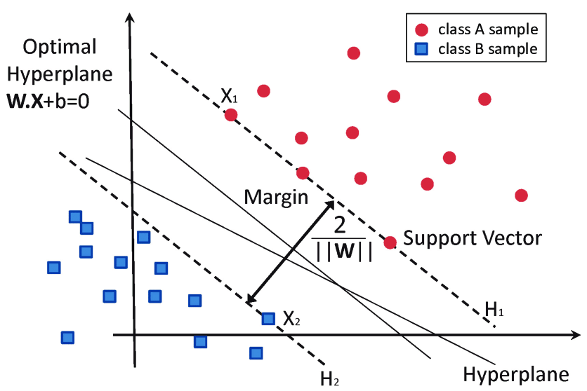
Image credit: García-Gonzalo et al. (2016)
Support Vector Machines (SVMs) are a powerful and versatile tool in machine learning, designed to tackle both linear and nonlinear classification problems. At their core, SVMs aim to find the optimal hyperplane that not only separates different classes but does so with the maximum margin. This margin, representing the smallest distance between the hyperplane and any data point, is key to SVM’s robustness and generalization capabilities.
In this blog, we'll delve into the essential components of SVMs, including:
- Calculating the distance from a point to a hyperplane and defining the margin.
- Formulating the hard-margin SVM and understanding how it finds the optimal separating hyperplane.
- Extending to soft-margin SVM to handle misclassifications and margin violations.
- Exploring the kernel trick, a powerful technique that enables SVMs to:
🔹 Efficiently classify complex, nonlinear data.
🔹 Map data into higher-dimensional spaces.
🔹 Avoid explicitly computing high-dimensional transformations.
Model Specification
Let be our training set, with and . We define:
- as the normal vector,
- as the bias,
- the margin as the minimum distance from the hyperplane to any data point.
In an SVM, the decision rule is given by the sign of . If , then , otherwise . This simple yet powerful model underlies the classification process.
Margin and Perfect Separation
Background: Distance from a Point to a HyperplaneIn three-dimensional space, the perpendicular distance from a point to a plane
is given by
Generalizing this to , consider the hyperplane
where is the normal vector and is the bias term. For any point , its perpendicular distance to this hyperplane is
Margin derivationFor a point with label , its signed distance to the hyperplane is
To ensure correct classification with a buffer (the margin), we impose
Under this scaling, the margin is
Thus, maximizing the margin reduces to minimizing (or for mathematical convenience).
Hard-Margin SVM
If the training data are perfectly separable, we can write the constraints as
Then the hard-margin SVM optimization problem is
Derivation of the Hinge Loss
In practice, data are rarely perfectly separable. To accommodate misclassifications or margin violations, we introduce slack variables . The modified constraint is
The slack variable quantifies how much the constraint is violated. If the constraint is met exactly or exceeded, then ; if not, is the shortfall. Then, this violation can be written as
This expression is known as the hinge loss:
It is zero when (i.e., when the data point is correctly classified with a sufficient margin) and increases linearly otherwise.
Soft-Margin SVM (Convex Optimization)
To build a formulation that penalizes margin violations, we incorporate the slack variables directly into the objective function. This is done using convex optimization by combining constraints and penalties into a single objective via a Lagrangian-type formulation. The resulting soft-margin SVM optimization problem is:
where is a parameter that balances the trade-off between maximizing the margin and minimizing the misclassification error.
Using our derivation of the hinge loss, we can equivalently express the penalty term as:
.
Thus, the soft-margin SVM optimization problem becomes:
Because the objective is convex, it can be solved via methods such as quadratic programming or gradient-based algorithms.
The Kernel Trick: Handling Nonlinear Boundaries
Some datasets cannot be well separated by a hyperplane in the original feature space. To address this, we map data into a (possibly high-dimensional) feature space using a transformation :
This notation is read as: “The function takes an input from the original -dimensional space and transforms it into a new representation in a higher-dimensional Hilbert space .” Here:
- is the original input space where our data lives.
- is a Hilbert space (often high-dimensional or even infinite-dimensional) in which the data may become linearly separable.
- The arrow indicates that each data point is transformed into .
In the feature space , the SVM decision function becomes
Directly computing might be impractical if is very large. Instead, we define a kernel function such that
This allows us to compute dot products in using only the original input vectors, avoiding explicit computation of . An RKHS (Reproducing Kernel Hilbert Space) is a Hilbert space of functions where point evaluation is continuous. This kernel function implicitly defines an RKHS (Reproducing Kernel Hilbert Space), where it acts as an inner product and provides the theoretical foundation for the kernel trick by ensuring that corresponds to an inner product in a high-dimensional space.
Primal and Dual Formulations of SVM
In optimization, the primal problem is the original formulation where we directly minimize an objective function over the decision variables subject to constraints. For example, a general constrained problem can be written as:
The dual problem is derived by introducing Lagrange multipliers to form a lower bound on the primal objective—this is done by taking the infimum of the Lagrangian over the primal variables. Under conditions such as convexity and Slater’s condition, strong duality holds, meaning the optimal values of the primal and dual problems are equal. In the case of a soft-margin SVM, the primal formulation seeks to determine the weight vector , bias , and slack variables to balance maximizing the margin and minimizing classification errors. Its objective is:
subject to
By introducing Lagrange multipliers for the margin constraints and for the slack constraints, we form the Lagrangian:
By differentiating the Lagrangian with respect to the primal variables and setting the derivatives to zero, we obtain the necessary optimality conditions known as the Karush-Kuhn-Tucker (KKT) conditions that must be satisfied at the optimal solution of the constrained problem. For the SVM problem, these KKT conditions are as follows:
Differentiating with respect to :
Differentiating with respect to :
Differentiating with respect to each :
Since , it follows that . This dual formulation expresses the optimization solely in terms of the Lagrange multipliers and inner products between data points, paving the way for the kernel trick.
Objective Function with a Kernel
To handle nonlinear boundaries, we map data into a high-dimensional feature space using a function , and define the kernel function . In this space, the soft-margin SVM primal objective becomes:
Here, the term controls the margin's width. Following the dual derivation, by enforcing the constraints with Lagrange multipliers and applying the KKT conditions, the weight vector in the feature space is expressed as:
Substituting this expression back into the norm term yields:
Thus, the kernelized dual formulation is:
subject to and . This derivation shows how the regularization in the primal problem is transformed into kernel evaluations in the dual, enabling SVMs to efficiently handle nonlinear boundaries without explicitly computing .
Examples of Common Kernels
- Polynomial Kernel: where , , and are hyperparameters.
- Radial Basis Function (RBF) Kernel: with controlling the spread.
-
What happens:
- In training, the dual formulation of the SVM uses only dot products, which are computed as .
- The final classifier depends solely on these kernel evaluations rather than on explicit high-dimensional feature vectors.
-
What does not happen:
- We do not build or store the high-dimensional vectors .
- We do not directly compute large dot products in the transformed space.
Recap
- Distance to Hyperplane:
- Margin:
Imposing leads to .
- Hard-Margin SVM:
- Hinge Loss:
- Soft-Margin SVM:
- Kernel Trick: which allows us to implicitly map data to a high-dimensional space without explicitly computing .
- Kernelized Dual Form: subject to and .