Nilson Chapagain

In the realm of binary classification, the ideal goal is to minimize the 0,1 loss, which simply assigns a penalty of 1 for every misclassified instance and 0 for a correct classification. Formally, if we denote the true label by $y \in \{-1,+1\}$ and the prediction by $\hat{y}$ , the 0,1 loss is defined as

L_{\text{0–1}}(y, \hat{y}) \;=\; \begin{cases} 0, & \text{if } y = \hat{y},\\[1mm] 1, & \text{if } y \neq \hat{y}. \end{cases}

In indicator notation, we can write this as

L_{\text{0–1}}(y,\hat{y}) \;=\; 1\{y \neq \hat{y}\}.

We often take $\hat{y} = \mathrm{sign}\bigl(f(x)\bigr)$ , where $f$ is often referred to as an estimator or a decision function or the learned model or hypothesis that maps input features $x$ to a real-valued score, with its sign used to determine the predicted class label.

When $y$ and $f(x)$ share the same sign, their product $y\,f(x)$ is positive (correct classification i.e. $y = \hat{y}$ ), whereas if their product is non-positive ( $y\,f(x) \le 0$ ), it indicates a misclassification i.e. $y \neq \hat{y}$ . Thus, defining $z = y\,f(x)$ , we penalize negative or zero $z$ , and the 0–1 loss can also be written as

L_{\text{0–1}}(z) =\; 1\{y \neq \hat{y}\} = 1\{ y\,f(x) \le 0 \} = 1\{ z \le 0 \}.

Despite its intuitive appeal, directly minimizing this loss is computationally challenging because it is both discontinuous and nonconvex. This difficulty has led researchers and practitioners to adopt more tractable alternatives known as surrogate loss functions.

The Role of Surrogate Loss Functions

Surrogate losses are designed to approximate the 0,1 loss while offering the advantages of smoothness and convexity, properties that make optimization via gradient based methods feasible. Some of the most popular surrogate losses include:

Hinge Loss: $\phi_{\text{hinge}}(z) = \max\{0,\,1 - z\}$ , famously used in Support Vector Machines.
Exponential Loss: $\phi_{\text{exp}}(z) = \exp(-z)$ , which is the backbone of AdaBoost.
Logistic Loss: $\phi_{\text{log}}(z) = \ln\bigl(1 + \exp(-z)\bigr)$ , a staple in logistic regression.
Truncated Quadratic Loss: $\phi_{\text{tquad}}(z)=\begin{cases}(1-z)^2,&z<1,\\0,&z\ge1.\end{cases}$ , behaves quadratically up to a certain margin and then flattens out.

In these expressions, $z = y\,f(x)$ represents the margin, a product of the true label $y$ and the scoring function $f(x)$ whose sign determines the classification.

Why Convexity Matters

Each surrogate loss is carefully chosen not only for its ease of optimization but also for its convexity. Convex functions are highly desirable in optimization because any local minimum is also a global minimum. Let us take a closer look at a few examples:

1. Hinge Loss

Defined as

\phi_{\text{hinge}}(z) = \max\{0,\,1 - z\},

the hinge loss is the pointwise maximum of the linear function $1-z$ and the constant function 0. We can break this down further:

\phi_{\text{hinge}}(z) = \begin{cases} 1 - z, & \text{if } z < 1,\\[1mm] 0, & \text{if } z \ge 1. \end{cases}

Why Convex?

Piecewise Definition:
For $z < 1$ , we have $\phi_{\text{hinge}}(z) = 1 - z$ , and for $z \ge 1$ , $\phi_{\text{hinge}}(z) = 0$ .
Convexity Criterion:
A function that is the maximum of two convex functions is itself convex. Here, the constant function 0 is convex, and $1-z$ is an affine (linear) function, which is convex. Thus, their pointwise maximum, $\phi_{\text{hinge}}(z)$ , is convex.
Conclusion:
Hence, $\phi_{\text{hinge}}(z) = \max\{0,\,1 - z\}$ is convex.

2. Exponential Loss

With the form

\phi_{\text{exp}}(z) = e^{-z},

the exponential loss is smooth and strictly convex. The details are as follows:

First Derivative: $\frac{d}{dz} \phi_{\text{exp}}(z) = \frac{d}{dz} \bigl(e^{-z}\bigr) = -\,e^{-z}.$
Second Derivative: $\frac{d^2}{dz^2} \phi_{\text{exp}}(z) = \frac{d}{dz} \bigl(-\,e^{-z}\bigr) = e^{-z}.$
Positivity of Second Derivative:
Since $e^{-z} > 0$ for all real $z$ , it follows that
$\frac{d^2}{dz^2} \phi_{\text{exp}}(z) > 0,$
which implies that $\phi_{\text{exp}}(z)$ is strictly convex.

3. Logistic Loss

The logistic loss is given by

\phi_{\text{log}}(z) = \ln\bigl(1 + e^{-z}\bigr).

We now elaborate its mathematical properties:

First Derivative:
Let $\alpha(z)=e^{-z}$ . Then,
$\phi_{\text{log}}'(z) = \frac{d}{dz} \ln\bigl(1 + \alpha(z)\bigr) = \frac{1}{1 + \alpha(z)} \cdot \frac{d}{dz}\bigl(1 + \alpha(z)\bigr) = \frac{-\,\alpha(z)}{1 + \alpha(z)}.$
Hence,
$\phi_{\text{log}}'(z) = -\,\frac{e^{-z}}{1 + e^{-z}}.$
Second Derivative:
Differentiating again,
$\phi_{\text{log}}''(z) = \frac{d}{dz} \Bigl(-\,\frac{e^{-z}}{1 + e^{-z}}\Bigr).$
A systematic approach is to set $\alpha(z)=e^{-z}$ (so that $\alpha'(z)=-e^{-z}=-\alpha(z)$ ) and apply the quotient rule. This yields:
$\phi_{\text{log}}''(z) = \frac{e^{-z}}{(1 + e^{-z})^2}.$
Positivity of Second Derivative:
Since both $e^{-z}$ and $(1 + e^{-z})^2$ are positive for all $z$ , we have:
$\phi_{\text{log}}''(z) > 0,$
confirming that $\phi_{\text{log}}(z)$ is strictly convex.

It is important to note that although the standard logistic loss evaluates to $\ln 2 \approx 0.693$ at $z=0$ , which is below the value 1 of the 0,1 loss, this does not affect its minimizer. Both the standard logistic loss and its scaled version (where it is multiplied by $1/\ln 2$ so that it equals 1 at $z=0$ ) yield the same optimal decision boundary. The scaled version is used in theoretical analyses to ensure that the surrogate loss majorizes the 0,1 loss.

4. Truncated Quadratic Loss

Often defined as

\phi_{\text{tquad}}(z) = \begin{cases} (1 - z)^2, & \text{if } z < 1,\\[1mm] 0, & \text{if } z \ge 1, \end{cases}

this loss function is constructed by taking the maximum of a quadratic function and 0. This approach ensures that the penalty is quadratic for $z < 1$ but does not grow unbounded for very confident predictions (i.e., when $z \ge 1$ ). Since both $(1-z)^2$ and 0 are convex, their maximum is also convex.

Fisher Consistency, Bridging Surrogate Losses and the 0,1 Loss

One critical requirement for any surrogate loss is Fisher consistency. A surrogate loss is Fisher consistent if minimizing the expected surrogate risk leads to the same decision boundary as minimizing the 0,1 loss in the limit of infinite data.

Consider the conditional probability $\eta(x) = P(Y=+1 \mid X=x)$ . The Bayes optimal classifier under the 0,1 loss is given by

h^*(x) = \begin{cases} +1, & \text{if } \eta(x) \ge 0.5, \\[1mm] -1, & \text{otherwise.} \end{cases}

When we define the surrogate risk as

R_\phi(f) = \mathbb{E}\bigl[\phi(Y \, f(X))\bigr],

Fisher consistency requires that the function $f^*$ which minimizes $R_\phi(f)$ also satisfies

\operatorname{sign}\bigl(f^*(x)\bigr) \;=\; \begin{cases} +1, & \text{if } \eta(x) > 0.5, \\ -1, & \text{if } \eta(x) < 0.5. \end{cases}

Thus, even though we are not minimizing the 0,1 loss directly, the surrogate risk leads us to the optimal classification rule as the amount of data grows.

Surrogate Losses as Upper Bounds

Surrogate loss functions are used not only because they are easier to optimize than the 0,1 loss but also because they provide an upper bound on the 0,1 loss. Recall that the 0,1 loss is defined as

L_{0\text{-}1}(z) = \mathbf{1}\{z \le 0\},

and the surrogate risk for a classifier $f$ is given by

R_\phi(f) = E_{(x,y)}[\phi(Y\,f(X))]\;=\; \int \phi\bigl(y\,f(x)\bigr)\,dP(x,y),

where $\phi$ is a convex surrogate loss function for the 0–1 loss.

Classification Calibration:

A surrogate loss $\phi$ is classification calibrated if there exists a function $\delta(\epsilon) > 0$ such that for any measurable function $f$ ,

R_{0\text{-}1}(f) - R_{0\text{-}1}^* \ge \epsilon \quad \Longrightarrow \quad R_\phi(f) - R_\phi^* \ge \delta(\epsilon),

where

R_{0\text{-}1}(f) = \mathbb{E}\bigl[\mathbf{1}\{\mathrm{sign}(f(X)) \neq Y\}\bigr]

is the misclassification error, $R_{0\text{-}1}^*$ is the Bayes risk (i.e. the minimum possible misclassification error), and $R_\phi(f)$ is the surrogate risk.

To express this pointwise, define the conditional risk at $x$ for the surrogate loss as

C_\phi(f(x)) = \eta(x)\,\phi(f(x)) + (1-\eta(x))\,\phi(-f(x)),

with $\eta(x)=P(Y=1|X=x)$ . A surrogate loss $\phi$ is classification calibrated if, for every $x$ with $\eta(x) \neq 1/2$ , any minimizer $f^*(x)$ of the conditional risk

C_\phi(f(x)) = E[\phi(Y\,f(x))|X=x]

satisfies

\mathrm{sign}(f^*(x)) = \mathrm{sign}(2\eta(x)-1).

Here’s how this ensures that lowering the surrogate risk will lead to lower misclassification error:

The inequality

R_{0\text{-}1}(f) - R_{0\text{-}1}^* \ge \epsilon \quad \Longrightarrow \quad R_\phi(f) - R_\phi^* \ge \delta(\epsilon)

tells us that if a classifier’s overall misclassification error is at least $\epsilon$ worse than the best achievable (Bayes risk), then its overall surrogate risk must be at least $\delta(\epsilon)$ worse than the optimal surrogate risk. Since $\delta(\epsilon)$ is strictly positive for any $\epsilon > 0$ , there is a quantifiable gap in surrogate risk whenever there is a gap in misclassification error. In practical terms, if you manage to reduce the surrogate risk (i.e. make $R_\phi(f)$ closer to $R_\phi^*$ ), then the corresponding misclassification error gap $R_{0\text{-}1}(f) - R_{0\text{-}1}^*$ must also decrease; otherwise, the surrogate risk gap would remain above the threshold given by $\delta(\epsilon)$ .

Therefore, Fisher consistency focuses on the theoretical, ideal alignment between the surrogate risk minimizer and the Bayes optimal decision rule (i.e. in the conditional risk sense, ensuring that for each $x$ , the best decision under the surrogate loss agrees with $\mathrm{sign}(2\eta(x)-1)$ ). In contrast, classification calibration provides a practical guarantee: it ensures that reducing the overall surrogate risk will directly lead to a reduction in the overall misclassification error. Thus, while both properties ensure that the surrogate loss guides us toward the Bayes optimal classifier, classification calibration explicitly links improvements in the surrogate risk with improved classification performance.

Below, we demonstrate this mathematically for the hinge loss.

Mathematical Demonstration for Hinge Loss

The hinge loss is defined as

\phi_{\text{hinge}}(z) = \max\{0,\,1 - z\},

which can be written in piecewise form as

\phi_{\text{hinge}}(z) = \begin{cases} 1 - z, & \text{if } z < 1,\\[1mm] 0, & \text{if } z \ge 1. \end{cases}

For a fixed $x$ , define the conditional risk associated with a surrogate loss $\phi$ as

C_\eta(\alpha) = \eta \, \phi(\alpha) + (1-\eta) \, \phi(-\alpha),

where $\alpha = f(x)$ and $\eta = \eta(x)$ .

For the hinge loss, assume $\alpha \in [-1,1]$ so that:

$\phi_{\text{hinge}}(\alpha) = 1 - \alpha$ (since $\alpha < 1$ ), and
$\phi_{\text{hinge}}(-\alpha) = 1 + \alpha$ (since $-\alpha < 1$ when $\alpha > -1$ ).

Then the conditional risk becomes:

\begin{aligned} C_\eta(\alpha) &= \eta \, (1 - \alpha) + (1-\eta) \, (1 + \alpha)\\[1mm] &= \eta + (1-\eta) - \eta \, \alpha + (1-\eta) \, \alpha\\[1mm] &= 1 + \alpha \, \bigl[(1-\eta) - \eta\bigr]\\[1mm] &= 1 + \alpha \, (1 - 2\eta). \end{aligned}

Now, analyze the behavior of $C_\eta(\alpha)$ :

If $\eta > 0.5$ , then $1 - 2\eta < 0$ , so $C_\eta(\alpha)$ is a decreasing function of $\alpha$ . Its minimum over $\alpha \in [-1,1]$ is achieved at $\alpha = 1$ .
If $\eta < 0.5$ , then $1 - 2\eta > 0$ , so $C_\eta(\alpha)$ is an increasing function of $\alpha$ . Its minimum is achieved at $\alpha = -1$ .
If $\eta = 0.5$ , then $C_{0.5}(\alpha) = 1$ for any $\alpha$ , meaning any $\alpha \in [-1,1]$ minimizes the risk.

Thus, the minimizer $\alpha^*(\eta)$ is:

\alpha^*(\eta) = \begin{cases} 1, & \text{if } \eta > 0.5,\\[1mm] -1, & \text{if } \eta < 0.5. \end{cases}

Taking the sign, we obtain:

\text{sign}\bigl(\alpha^*(\eta)\bigr) = \text{sign}(2\eta - 1),

which is exactly the Bayes optimal decision rule under the 0,1 loss. Therefore, minimizing the hinge loss is Fisher consistent.

Mathematical Demonstration for Logistic Loss

The logistic loss is defined as

\phi_{\text{log}}(z) = \ln(1 + e^{-z}).

For a fixed $x$ , define the conditional risk associated with a surrogate loss $\phi$ as

C_\eta(\alpha) = \eta \, \phi(\alpha) + (1-\eta) \, \phi(-\alpha),

where $\alpha = f(x)$ and $\eta = \eta(x) = P(Y = +1 \mid X = x)$ .

For the logistic loss, this becomes

C_\eta(\alpha) = \eta \ln(1 + e^{-\alpha}) + (1-\eta) \ln(1 + e^{\alpha}).

To find the minimizer $\alpha^*(\eta)$ , differentiate $C_\eta(\alpha)$ with respect to $\alpha$ and set the derivative equal to zero.

Differentiate the first term:
The derivative of $\ln(1 + e^{-\alpha})$ with respect to $\alpha$ is
$\frac{d}{d\alpha} \ln(1 + e^{-\alpha}) = -\frac{e^{-\alpha}}{1 + e^{-\alpha}}.$
Differentiate the second term:
Similarly, the derivative of $\ln(1 + e^{\alpha})$ with respect to $\alpha$ is
$\frac{d}{d\alpha} \ln(1 + e^{\alpha}) = \frac{e^{\alpha}}{1 + e^{\alpha}}.$

Thus, the derivative of the conditional risk is

C_\eta'(\alpha) = \eta \left(-\frac{e^{-\alpha}}{1 + e^{-\alpha}}\right) + (1-\eta) \left(\frac{e^{\alpha}}{1 + e^{\alpha}}\right).

Setting $C_\eta'(\alpha) = 0$ , we obtain

-\eta \frac{e^{-\alpha}}{1 + e^{-\alpha}} + (1-\eta) \frac{e^{\alpha}}{1 + e^{\alpha}} = 0.

With some algebraic manipulation (multiplying numerator and denominator appropriately or recognizing standard forms), one can show that the solution to this equation is

\alpha^*(\eta) = \ln \frac{\eta}{1-\eta}.

Now, observe the sign of $\alpha^*(\eta)$ :

If $\eta > 0.5$ , then $\frac{\eta}{1-\eta} > 1$ , so $\alpha^*(\eta) > 0$ .
If $\eta < 0.5$ , then $\frac{\eta}{1-\eta} < 1$ , so $\alpha^*(\eta) < 0$ .
If $\eta = 0.5$ , then $\alpha^*(\eta) = \ln 1 = 0$ .

Thus,

\text{sign}\bigl(\alpha^*(\eta)\bigr) = \text{sign}\left(\ln \frac{\eta}{1-\eta}\right) = \text{sign}(2\eta-1),

which is exactly the Bayes optimal decision rule under the 0,1 loss.

Therefore, minimizing the logistic loss is Fisher consistent, because it leads to the same decision boundary as minimizing the 0,1 loss.

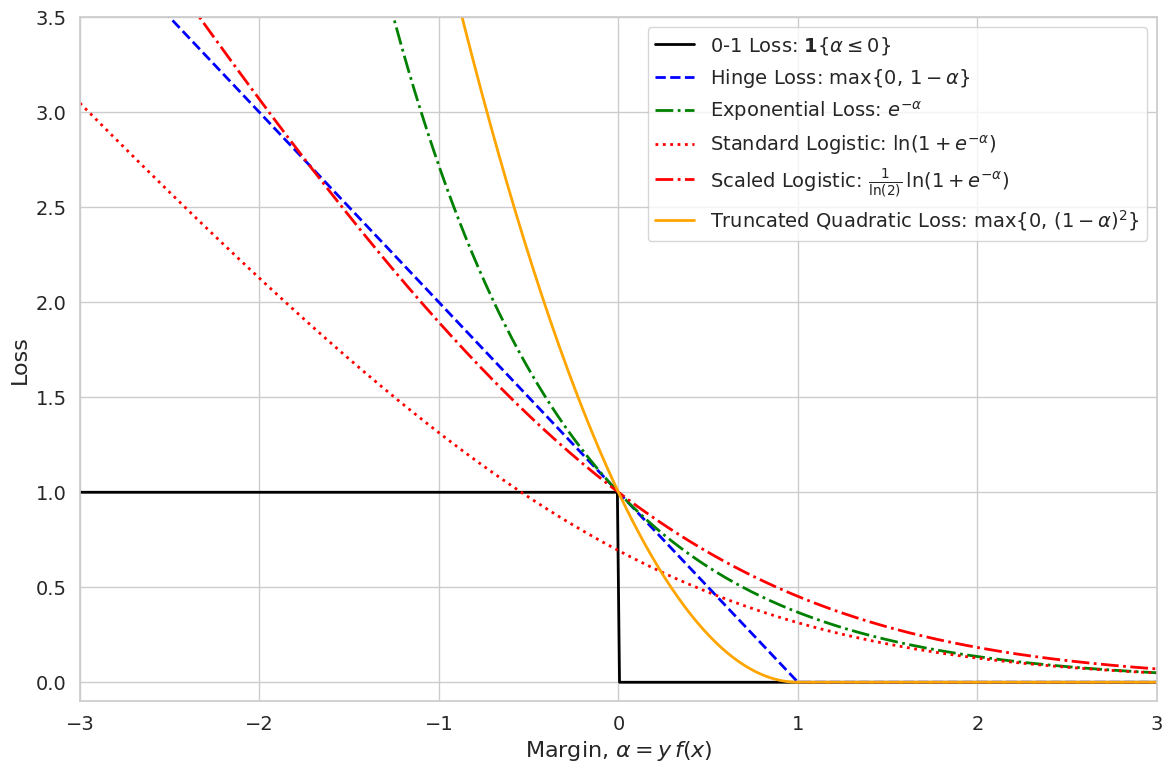
Visual Interpretation

Refer to the plot above where the 0,1 loss is depicted as a step function that jumps from 0 to 1 at $z=0$ . Overlaying this step function, the following surrogate curves are displayed:

Hinge Loss: Defined as $\max\{0,\,1-z\}$ , this piecewise linear curve increases linearly for $z<1$ and is 0 for $z \ge 1$ . It is favored for its simplicity and the ease with which it can be optimized.
Exponential Loss: Given by $e^{-z}$ , this smooth curve decays exponentially as $z$ increases, thereby penalizing misclassified examples with a low margin quite heavily.
Standard Logistic Loss: This is expressed as $\ln(1+e^{-z})$ . Note that at $z=0$ , it evaluates to $\ln 2 \approx 0.693$ , which lies below the 0,1 loss value of 1. However, despite this pointwise difference, both the standard logistic loss and any suitably scaled version yield the same minimizer due to the property of classification calibration.
Scaled Logistic (Deviance): To obtain a curve that majorizes the 0,1 loss, the logistic loss is often scaled by a factor of $1/\ln 2$ . This scaled version, $\frac{1}{\ln 2}\ln(1+e^{-z}),$ attains the value 1 at $z=0$ and lies entirely above the 0,1 loss for $z \le 0$ . The scaling does not change the minimizer of the surrogate risk but is useful for theoretical guarantees that the surrogate risk upper bounds the misclassification error ( $R_{0\text{-}1}(f) = \mathbb{E}\bigl[\mathbf{1}\{\mathrm{sign}(f(X)) \neq Y\}\bigr]$ ).
Truncated Quadratic Loss: Defined as $(1-z)^2$ for $z < 1$ and 0 for $z \ge 1$ , this loss combines a quadratic penalty with a truncation to avoid excessive punishment for high-margin points.

The key point is that although the standard logistic loss may be below the 0,1 loss at $z=0$ , its classification-calibrated property ensures that minimizing its risk leads to the same optimal classifier as minimizing the 0,1 loss. In contrast, the scaled logistic loss (or deviance) is adjusted to lie above the 0,1 loss, making it a strict upper bound in that region. This property is crucial for deriving theoretical risk bounds and for ensuring that the surrogate risk is a faithful proxy for the true misclassification error.

Key Takeaways:

0,1 Loss and Its Challenges: The 0,1 loss is the most natural measure of misclassification but is nonconvex and discontinuous, making it computationally intractable for direct optimization.
Surrogate Loss Functions: Surrogates such as hinge, exponential, logistic, and truncated quadratic losses offer smooth and convex approximations that greatly simplify the optimization process. Their forms can be further adjusted, for example by scaling, to ensure they majorize the 0,1 loss.
Fisher Consistency: A key property of these surrogate losses is classification calibration. This means that even if the surrogate’s pointwise values differ from the 0,1 loss (as seen with the standard logistic loss), minimizing the surrogate risk ultimately yields the same decision boundary as minimizing the 0,1 loss.
Upper Bound Nature: By appropriately scaling (e.g., multiplying the logistic loss by $1/\ln(2)$ ), surrogate losses can be made to serve as strict upper bounds on the 0,1 loss. This theoretical guarantee is critical for deriving risk bounds and ensuring that optimizing the surrogate risk indirectly minimizes the true classification error.
Optimization and Theoretical Guarantees: The convexity of these surrogate losses not only enables efficient gradient-based optimization but also provides robust theoretical guarantees that the surrogate risk is closely aligned with the true misclassification risk.

Surrogate loss functions play a pivotal role in modern machine learning by bridging the gap between computational tractability and statistical optimality. While the 0,1 loss is the most intuitive measure of classification error, its nonconvex and discontinuous nature renders it impractical for optimization. In contrast, surrogate losses—such as the hinge, exponential, logistic, and truncated quadratic losses—provide smooth and convex alternatives that are far easier to minimize. Importantly, these surrogates are designed to be Fisher consistent; that is, they ensure that minimizing the surrogate risk yields the same optimal decision boundary as the 0,1 loss in the infinite-sample limit. Moreover, by scaling losses like the logistic loss (resulting in the deviance), we can enforce that the surrogate not only approximates but strictly upper-bounds the 0,1 loss in the region of interest. This property is crucial for both practical algorithm performance and the derivation of rigorous theoretical risk bounds. Ultimately, the careful selection and scaling of surrogate losses enable practitioners to harness the power of convex optimization while accurately approximating the ultimate goal of minimizing misclassification error.