Linear Regression: OLS, Ridge, Lasso & Elastic Net

Linear regression is a foundational technique in both classical statistics and machine learning, offering a straightforward method for modeling relationships between variables. However, real-world data often present challenges such as overfitting and multicollinearity, which can compromise the predictive performance and stability of the model. This article covers the Frequentist derivation (through minimizing squared errors or equivalently maximizing likelihood) for Ordinary Least Squares (OLS) and then explores key regularization variants such as Ridge, Lasso, and Elastic Net. Finally, we discuss the assumptions behind linear regression and strategies to check them.

Key Regression Framework

Frequentist Approach

Frequentist (or “classical”) linear regression treats the parameters $\boldsymbol{\beta}$ as fixed but unknown quantities. We usually assume a linear relationship between the predictors and the response, along with normally distributed errors:

y_i = \beta_0 + \beta_1 x_{i1} + \dots + \beta_p x_{ip} + \epsilon_i,

where each $\epsilon_i \sim N(0,\, \sigma^2)$ . In compact matrix notation, this becomes:

\mathbf{y} = \mathbf{X}\boldsymbol{\beta} + \boldsymbol{\epsilon},

with $\mathbf{y}$ as an $n \times 1$ response vector, $\mathbf{X}$ as an $n \times (p+1)$ design matrix, $\boldsymbol{\beta}$ as the $(p+1) \times 1$ vector of unknown coefficients, and the errors $\boldsymbol{\epsilon} \sim N(\mathbf{0}, \sigma^2 \mathbf{I})$ .

Estimating Parameters (OLS & MLE)

To estimate $\boldsymbol{\beta}$ , the Frequentist approach typically uses the Ordinary Least Squares (OLS) criterion, which minimizes the sum of squared residuals (SSR), also known as the Residual Sum of Squares (RSS). Mathematically, the RSS is given by:

RSS = \sum_{i=1}^{n} (y_i - \hat{y}_i)^2 = (\mathbf{y} - \mathbf{X}\boldsymbol{\beta})^T(\mathbf{y} - \mathbf{X}\boldsymbol{\beta}) = \|\mathbf{y} - \mathbf{X}\boldsymbol{\beta}\|_2^2.

Diagram illustrating the Residual Sum of Squares (RSS) for a linear regression

Image credit: Article by wallstreetmojo

In the plot, each data point $(x_i, y_i)$ has a corresponding predicted value $\hat{y}_i$ . The vertical lines (labeled $e_1, e_2, \dots$ ) represent the residuals, mathematically given by $e_i = y_i - \hat{y}_i$ . The Residual Sum of Squares (RSS) is the sum of the squares of these residuals, i.e., $RSS = \sum_{i=1}^{n} e_i^2.$ Minimizing the RSS via Ordinary Least Squares (OLS) gives us the estimate for $\beta$ .

Under the normal error assumption, maximizing the likelihood function is equivalent to minimizing the RSS. This procedure gives a single “best-fit” solution for $\boldsymbol{\beta}$ , in contrast to the Bayesian approach, which produces a full posterior distribution over possible values of $\boldsymbol{\beta}$ .

Deriving OLS and MLE Estimates for Linear Regression

Model Setup

We consider $\mathbf{y} = \mathbf{X}\boldsymbol{\beta} + \boldsymbol{\epsilon}$ , where $\boldsymbol{\epsilon} \sim N(0, \sigma^2 \mathbf{I})$ .

Here, $\mathbf{X}$ is an $n \times (p+1)$ design matrix, $\mathbf{y}$ is an $n \times 1$ vector, and $\boldsymbol{\beta}$ is a $(p+1) \times 1$ vector of unknown parameters.

1. OLS Estimation (Loss Function Approach)

Define the Loss Function

S(\boldsymbol{\beta}) = \|\mathbf{y} - \mathbf{X}\boldsymbol{\beta}\|^2 = (\mathbf{y} - \mathbf{X}\boldsymbol{\beta})^T(\mathbf{y} - \mathbf{X}\boldsymbol{\beta})

Take the Derivative

\frac{\partial S(\boldsymbol{\beta})}{\partial \boldsymbol{\beta}} = -2\mathbf{X}^T\mathbf{y} + 2\mathbf{X}^T\mathbf{X}\boldsymbol{\beta} = 0

Solve for $\boldsymbol{\beta}$

\mathbf{X}^T\mathbf{X}\boldsymbol{\beta} = \mathbf{X}^T\mathbf{y} \\ \implies \hat{\boldsymbol{\beta}_{OLS}} = (\mathbf{X}^T\mathbf{X})^{-1}\mathbf{X}^T\mathbf{y}

2. MLE Estimation (Likelihood Approach)

Likelihood Definition

Under $\boldsymbol{\epsilon} \sim N(0, \sigma^2 \mathbf{I})$ , the probability density of $\mathbf{y}$ given $\boldsymbol{\beta}$ and $\sigma^2$ is:

p(\mathbf{y} \mid \boldsymbol{\beta}, \sigma^2) = \frac{1}{(2\pi\sigma^2)^{n/2}} \exp\left(-\frac{1}{2\sigma^2} \|\mathbf{y} - \mathbf{X}\boldsymbol{\beta}\|^2\right)

Log-Likelihood

Taking the natural log:

\ell(\boldsymbol{\beta}, \sigma^2) = -\frac{n}{2}\ln(2\pi) - \frac{n}{2}\ln(\sigma^2) - \frac{1}{2\sigma^2} \|\mathbf{y} - \mathbf{X}\boldsymbol{\beta}\|^2

Maximizing with Respect to $\boldsymbol{\beta}$

Focus on the term $-\frac{1}{2\sigma^2}\|\mathbf{y} - \mathbf{X}\boldsymbol{\beta}\|^2,$ which is the only component dependent on $\boldsymbol{\beta}$ . Maximizing this expression is equivalent to minimizing its negative: $\frac{1}{2\sigma^2}\|\mathbf{y} - \mathbf{X}\boldsymbol{\beta}\|^2.$ Since $\frac{1}{2\sigma^2}$ is a positive constant, minimizing this term is exactly the same as minimizing $\|\mathbf{y} - \mathbf{X}\boldsymbol{\beta}\|^2.$

Notice that maximizing the term $-\frac{1}{2\sigma^2}\|\mathbf{y} - \mathbf{X}\boldsymbol{\beta}\|^2$ is equivalent to minimizing the Residual Sum of Squares (RSS), defined as $RSS = \|\mathbf{y} - \mathbf{X}\boldsymbol{\beta}\|^2$ . The objective functions for MLE and OLS are exactly the same because of the assumption of normally distributed errors, and minimizing this term yields the same estimates for $\boldsymbol{\beta}$ . This is why the Maximum Likelihood Estimation (MLE) criterion coincides with the Ordinary Least Squares (OLS) approach.

\frac{\partial}{\partial \boldsymbol{\beta}} \|\mathbf{y} - \mathbf{X}\boldsymbol{\beta}\|^2 = -2\mathbf{X}^T\mathbf{y} + 2\mathbf{X}^T\mathbf{X}\boldsymbol{\beta} = 0 \\ \implies \mathbf{X}^T\mathbf{X}\boldsymbol{\beta} = \mathbf{X}^T\mathbf{y} \\ \implies \hat{\boldsymbol{\beta}}_{\text{MLE}} = (\mathbf{X}^T\mathbf{X})^{-1}\mathbf{X}^T\mathbf{y}

In many regression problems, the standard OLS solution can result in overly complex models with large, unstable coefficients—particularly when the data contains noise or the predictors are highly correlated. To address these issues, we add constraints on the coefficient vector. By formulating the problem as one of constrained optimization and then applying the method of Lagrange multipliers, we convert these constraints into penalty terms in the objective function. This not only shrinks the coefficients to avoid overfitting but, in cases such as Lasso and Elastic Net, it can also force some coefficients exactly to zero, thereby performing variable selection. While all methods aim to prevent overfitting and achieve a favorable bias-variance trade-off, each approach does so in a distinct way: Ridge shrinks coefficients toward zero (but rarely to zero), Lasso shrinks some coefficients exactly to zero for variable selection, and Elastic Net combines both effects.

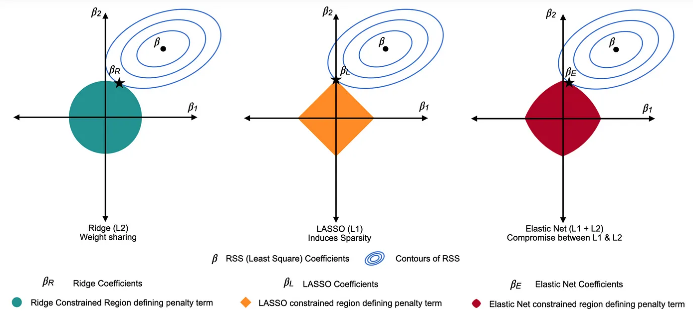
Diagram illustrating Ridge, Lasso, and Elastic Net regularization techniques for linear regression

Image credit: Article by Tavishi

Interpreting the Contours and Constrained Regions

Unconstrained Optimization (OLS Only):
You can think of the contour lines as slices of a “bowl” representing equal values of the residual sum of squares (RSS). Finding the minimum of the RSS is like locating the bottom of the bowl. In a 2D example (for $beta_1$ and $beta_2$ ), this minimum appears at the center of the smallest contour, where the slope is zero and the loss is minimized.

Constrained Optimization (Regularization):
Now, imagine placing a "plate" on top of the bowl to represent the constraint region imposed by regularization. For Ridge, this plate is circular; for Lasso, it's diamond-shaped; and for Elastic Net, it's a blend of both. The final solution is the point within this plate where the loss is minimum or the lowest — that is, the lowest point of the bowl that still lies within the boundaries of the plate. In other words, it’s where the smallest contour that is feasible (i.e., within the constraint region) touches the plate.

As the number of parameters grows, these geometric shapes extend to higher dimensions, but the principle remains the same: the optimum is found where the contours of the loss (the “higher dimensional bowl”) intersect with the constraint region (the “higher dimensional plate”).

Next, we will delve into the mathematical form of these regularization objectives. This section will illustrate Constrained formulation and the associated Objective or loss function using the Lagrangian formulation, and will discuss the key properties of each penalty.

Ridge Regression

Constrained Formulation:
$\min_{\boldsymbol{\beta}} \|\mathbf{y} - \mathbf{X}\boldsymbol{\beta}\|^2$ subject to $\|\boldsymbol{\beta}\|_2^2 \le t$ .
Using Lagrange multipliers, this converts to the penalized objective below.

Objective: Minimize
$\|\mathbf{y} - \mathbf{X}\boldsymbol{\beta}\|^2 + \lambda \|\boldsymbol{\beta}\|_2^2$

Closed-form Estimate:
$\hat{\boldsymbol{\beta}}_{\text{ridge}} = (\mathbf{X}^T\mathbf{X} + \lambda \mathbf{I})^{-1}\mathbf{X}^T\mathbf{y}$

Key Points for Ridge:

Coefficient Shrinkage: Ridge regression shrinks all coefficients toward zero by adding a quadratic penalty. This reduces their magnitude smoothly without setting any exactly to zero, which is beneficial when all predictors contribute information.
Handling Multicollinearity: The addition of $\lambda \mathbf{I}$ improves the conditioning of $\mathbf{X}^T\mathbf{X}$ , yielding more stable estimates in the presence of highly correlated predictors.
Overfitting Prevention: By shrinking coefficients, ridge reduces the risk of fitting noise, thereby enhancing the model's predictive performance.

Lasso Regression

Constrained Formulation:
$\min_{\boldsymbol{\beta}} \|\mathbf{y} - \mathbf{X}\boldsymbol{\beta}\|^2$ subject to $\|\boldsymbol{\beta}\|_1 \le t$ .
Using Lagrange multipliers, this constrained problem becomes the penalized objective below.

Objective: Minimize
$\|\mathbf{y} - \mathbf{X}\boldsymbol{\beta}\|^2 + \lambda \|\boldsymbol{\beta}\|_1$

Estimation: No closed-form solution; solved via numerical methods.

Key Points for Lasso:

Sparsity Induction: The $L_1$ penalty forces some coefficients to become exactly zero, effectively performing variable selection and yielding a more interpretable model.
Feature Selection: By eliminating less important predictors, lasso simplifies the model, which can be particularly useful in high-dimensional settings.
Overfitting Prevention: Shrinks coefficients while potentially removing irrelevant features entirely.

Elastic Net Regression

Constrained Formulation:
$\min_{\boldsymbol{\beta}} \|\mathbf{y} - \mathbf{X}\boldsymbol{\beta}\|^2$ subject to $\|\boldsymbol{\beta}\|_1 \le t_1$ and $\|\boldsymbol{\beta}\|_2^2 \le t_2.$

Formulation Approach:
Elastic Net integrates constraints on both the $L_1$ and $L_2$ norms via the Lagrangian method, leading to a combined penalized objective.

Objective: Solve
$\min_{\boldsymbol{\beta}} \; \|\mathbf{y} - \mathbf{X}\boldsymbol{\beta}\|^2 + \lambda_1 \|\boldsymbol{\beta}\|_1 + \lambda_2 \|\boldsymbol{\beta}\|_2^2$

Key Points for Elastic Net:

Dual Regularization: Combines the smooth shrinkage of ridge ( $L_2$ ) with the sparsity-inducing effect of lasso ( $L_1$ ), effectively balancing both worlds.
Group Selection: Particularly useful when predictors are highly correlated, as it tends to select groups of related variables.
Flexible Tuning: Offers additional flexibility by tuning two penalty parameters, allowing for a more nuanced control over model complexity.

Model Assumptions & How to Check Them

Linearity

Assumption: The relationship between the independent variables and the dependent variable is linear.

How to Check: Examine scatterplots of observed versus predicted values and plot each predictor against the residuals. A random scatter around zero suggests that the linearity assumption is met. Additionally, component-plus-residual (partial residual) plots can help detect nonlinearity.

Independence of Errors

Assumption: The residuals (errors) are assumed to be independent, meaning the error for one observation should not be correlated with the error for another.

How to Check: Inspect residual plots for any patterns or clusters that might indicate correlation among errors. While tests like the Durbin-Watson test are more common in time series, they can provide a rough check in cross-sectional data. Additionally, consider the study design to ensure observations were collected independently.

Homoscedasticity

Assumption: The variance of the errors should be constant across all levels of the independent variables.

How to Check: Plot the residuals versus the fitted values. A random scatter with a constant spread (and no funnel shape) suggests homoscedasticity. Formal tests such as the Breusch-Pagan or White’s test can also be used to assess constant variance.

Normality of Errors

Assumption: The residuals are assumed to be normally distributed, which is important for reliable hypothesis testing and constructing confidence intervals.

How to Check: Generate a Q-Q plot and a histogram of the residuals. If the residuals lie approximately along the 45-degree line in the Q-Q plot, the normality assumption is supported. You can also use formal tests such as the Shapiro-Wilk test for a more rigorous assessment.

No Multicollinearity

Assumption: The independent variables should not be too highly correlated, ensuring that each predictor provides unique information.

How to Check: Evaluate the correlation matrix of the independent variables and calculate Variance Inflation Factors (VIF). High correlations or VIF values above 5 (or 10, depending on the context) indicate potential multicollinearity issues.

Correct Model Specification

Assumption: The model should include all relevant predictors to avoid omitted variable bias, and exclude irrelevant ones.

How to Check: Review residual plots for systematic patterns that might indicate omitted variables or an incorrect functional form. Use information criteria such as AIC or BIC, perform specification tests, or apply stepwise selection methods to assess if the model is appropriately specified.

Regression Diagnostics

The most common approach is to apply the plot() function in R to the object returned by lm(). Doing so produces four graphs that are useful for evaluating the model fit.

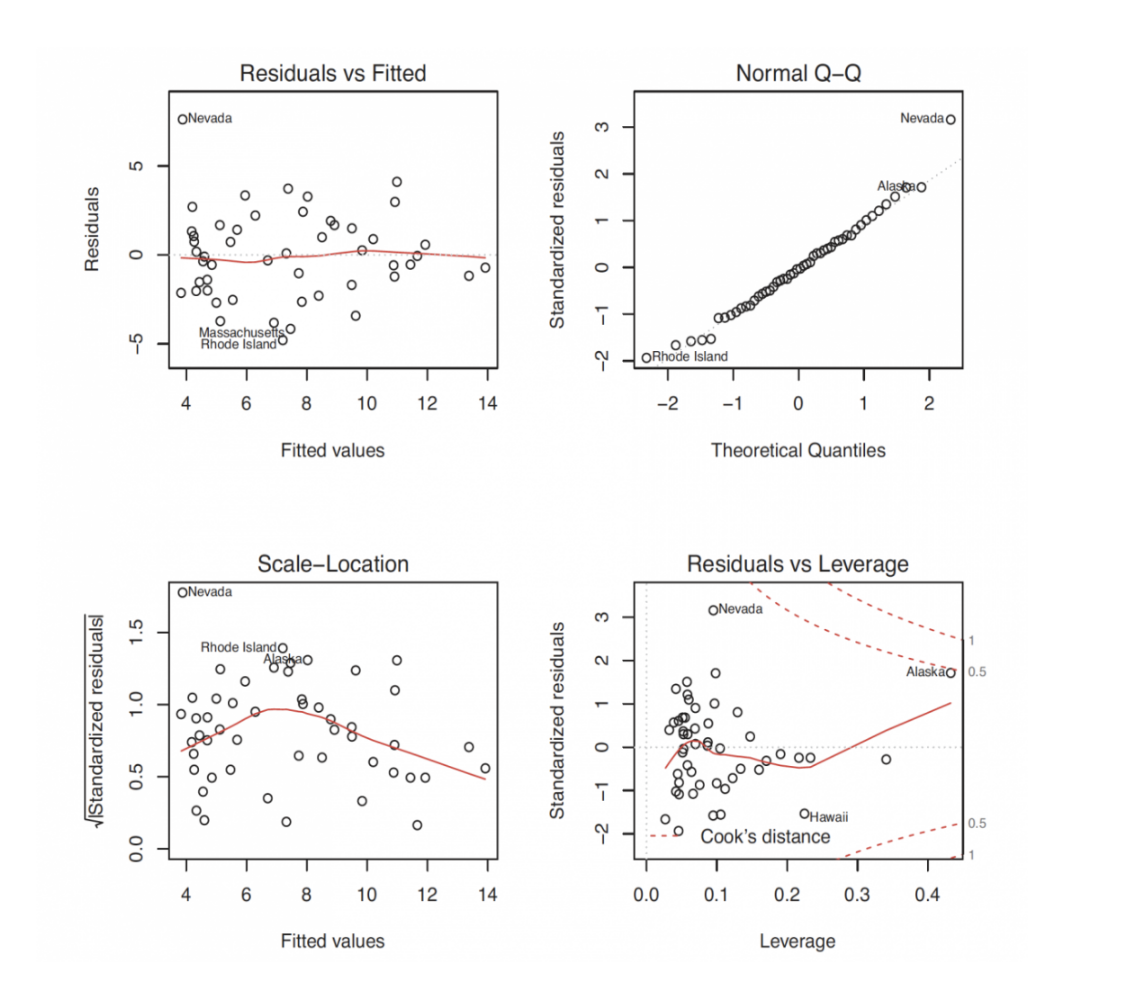
Support vector machine graphical representation

Residuals vs Fitted Plot

This plot displays the residuals on the vertical axis against the fitted values on the horizontal axis. Ideally, if the dependent variable is linearly related to the independent variables, the residuals should be randomly scattered around zero without any systematic pattern.

Assumption Checked: Linearity. A random scatter supports the linearity assumption, whereas a curved or patterned distribution suggests that a non-linear relationship might exist and that the model may need additional terms.

Normal Q-Q Plot

This plot compares the standardized residuals to the theoretical quantiles of a normal distribution. If the residuals are normally distributed, the points should align closely along a 45-degree line.

Assumption Checked: Normality of Errors. Deviations from the 45-degree line indicate departures from normality, which may affect hypothesis testing and confidence interval accuracy.

Scale-Location Plot

This plot shows the square root of the standardized residuals versus the fitted values. A random and even spread of points across the range of fitted values indicates that the variance of the errors remains constant.

Assumption Checked: Homoscedasticity. A horizontal band with no clear pattern supports the constant variance assumption; any funnel shape or systematic pattern suggests heteroscedasticity.

Residuals vs Leverage Plot

This plot helps identify influential observations by displaying residuals against leverage, which indicates the impact of each data point on the fitted model. Points that combine high leverage with large residuals may disproportionately affect the model's performance.

Assumption Checked: Although this plot is primarily used to detect influential observations, it also indirectly supports the independence assumption by revealing if a few cases are driving the model. In cross-sectional data, independence is generally inferred from the study design.

From the classic Frequentist OLS derivation to extensions like Ridge, Lasso, and Elastic Net, linear regression remains a fundamental tool in statistics and data science. These methods add regularization to combat overfitting, improve numerical stability, and, in the case of Lasso and Elastic Net, enhance model interpretability through variable selection. Always verify model assumptions with diagnostic tools and residual analyses to ensure valid inferences.